3.4: Determining the Brightness of Astronomical Objects

WHAT DO YOU THINK: WHAT ARE PHOTONS?

Members of the Stargazers Club are talking about their readings for class.

• Jennifer: Our book says that photometry is about counting photons—but what does that mean? What’s a photon? Is it like a proton?
• Lily: Photons are light so I think the number of photons has to do with how bright the object is.
• Mallory: I think a digital camera must have some way to count them.

Whether our telescopes are here on Earth or in space, we can only measure the light that hits our detectors. This process tells us how bright an object appears to be, and astronomers call this apparent brightness the flux or intensity. The measured flux is different from the object’s true inherent brightness, called its luminosity. The flux is just the energy we measure at a particular point in space in a given time, while the luminosity is the object’s total power output, measured in watts. Flux and luminosity are related in a way that you are probably familiar with from everyday life: If something is farther away, it will look dimmer, and if it is closer, it will look brighter. This is true no matter how bright an object is intrinsically: moving farther away from it will always make it appear dimmer. Here, you will learn how to measure the fluxes of sources using a CCD detector.

A CCD detector is composed of an array of rows and columns of individual light-sensitive elements, or pixels. One way to think of the pixels is as tiny buckets that collect photons, sort of the way rain buckets might catch raindrops during a storm. An incoming photon of light strikes the detector and produces electrons that are stored in the detector until they are read out. Built-in electronics organize these electrons as charge packets, and a computer can display and record them as a digital image. The resulting digital image is composed of numbers that correspond to the relative numbers of electrons stored in a given pixel, and thus the number of photons that struck that pixel. These numbers are generally called the “pixel values.” Figure 3.12 is a schematic representation of a detector with X columns and Y rows.

Figure 3.12: A CCD array is a grid of pixels, here numbered starting from the lower left. Each pixel is a mini light detector, storing electric charge in proportion to the number of photons that hit it. It is a bit like having buckets set out in a grid to catch rain: Each bucket will fill in proportion to the number of raindrops that fall into it. The pattern of charge on the array is what produces an image when the charge is read out by the camera circuitry. Credit: NASA/SSU/Kevin McLin.

Even though stars are technically point sources of light, an image of a star will have some physical size due to the blurring by Earth’s atmosphere, as well as by the diffraction and interference of the light waves (due to the telescope’s optics) that produce the image. A real star image will appear as a so-called seeing disk (see Figures 3.13, 3.14, and 3.15). This pattern will be brighter at the center of the disk and approach the sky background level at the edges of the pattern. Because of this blurring of stellar images, bright stars are represented by larger disks of light than faint stars on an image. That does not mean that the bright stars are necessarily bigger than fainter ones. In fact, they could be much smaller; we cannot tell just from the seeing disk.

Figure 3.13: An image displayed in a popular software package. The stars are the bright circles and the sky background is dark in this example. The “bigger” stars are actually just brighter than the “small” stars. All stars are unresolved point sources in this image. The stars are actually collections of square-shaped pixels, as can be seen in Figures 3.14 and 3.15. Credit: NASA/SSU/Kevin McLin.

It can be useful to visualize a digital star image in terms of a three-dimensional histogram of pixel values (see Figure 3.14). Here, the height corresponds to the value at a particular pixel and the rows and columns correspond to the location on the detector. In this representation, taller places represent larger pixel values—a brighter part of the image.

Figure 3.14: This plot displays the image brightness along a vertical axis above the pixel array. Each pixel contains a different number of counts, corresponding to the number of photons that landed in that pixel, and therefore, to the brightness of that part of the image. Notice how in this image, which is a star, the center is quite bright, and the edges gradually fall off to the sky background level. The width of the star is not zero, even though stars are technically point sources. The width of point sources is caused by optical effects in the telescope, as discussed in the text. Credit: NASA/SSU/Tim Graves.

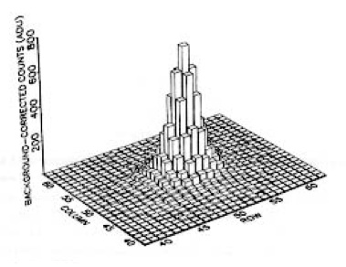
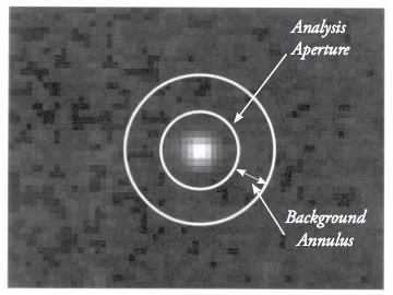
Figure 3.15 shows a highly magnified digital image of a real star. Notice that you can see the individual pixels in the star image, as well as in the sky background around the star. The inner circle represents the region within which nearly all the light from the star has struck the detector. For determining the brightness of an object, this circle is termed the analysis aperture. If we add up all the pixel values in the analysis aperture, we will have a number that represents the brightness of the star. This number is directly related to the number of photons coming from the star that struck the detector during the time the exposure was being made.

Figure 3.15: This image shows a star surrounded by the apertures used to measure its brightness. The inner aperture is the analysis aperture. It is assumed that all of the star’s light falls within this aperture, though that is not absolutely true. The outer circle sets the outer limit of the background annulus. In this region, the sky background is determined. More commonly, a third circle is used, and the annulus between the second and third circles is used to measure the sky background. Notice the pixelation of the image. Credit: NASA/SSU/Tim Graves.

When making a measurement of a star’s brightness, we must be careful to correct for any other sources of light. These light sources can contaminate the values of the star brightness. Spurious sources include light from the sky and from the detector itself. Together, these are called background counts. Even under the most ideal circumstances, the sky is never truly dark. There is always at least a small amount of light. In an urban or even a suburban environment, light pollution from artificial light sources will illuminate dust and molecules in the atmosphere. The atmosphere itself emits some light, resulting from interactions with solar wind particles. Another source is the integrated light from faint and distant stars - even Hubble cannot escape this background source. All of these sources from the sky are recorded by the detector and are collectively called the sky brightness.

Other important background sources results from the detector itself. The act of reading out the array introduces "read noise." This is from fluctuations in the count levels measured that are intrinsic to the camera and its electronics. Even in the total absence of light, a detector will produce electrons that get placed into the pixels. These are called the dark current of the detector and are caused by thermal motions (on the atomic level) of its internal components. Cooling the detector can almost completely negate this source of background counts.

To accurately measure the brightness of an astronomical object, the observer must correct for all these background counts (as well as several other sources of noise). The background annulus, formed by the inner and outer circles in Figure 3.15, is a region we can use to estimate the average background sky brightness reaching each pixel. The dark current can be determined by taking an exposure while the camera shutter is kept closed, thus only accumulating dark current since no light reaches the detector. The read noise is a more or less constant value for a given camera and need only be measured one time and then applied whenever the camera is used. These corrections can then be employed to adjust the counts obtained from the analysis aperture so that only the counts from the star are tallied.

GOING FURTHER 3.6: THE MAGNITUDE SYSTEM

In optical light, astronomers measure the brightness of astronomical objects using the magnitude system. Historically, the magnitude system is based on a concept first introduced by the Greek astronomer Hipparchus (c. 190 BCE–120 BCE). In about 129 BCE, Hipparchus produced the first well-known star catalog in the western world. In this catalog, Hipparchus ranked stars by what he called magnitude. He called the brightest stars he could see those of the first magnitude. Stars not so bright he called second magnitude. Using this system, he called the faintest stars he could just barely see sixth magnitude. This basic system has survived to today. Galileo forced us to change the system slightly. In 1610, when he used a telescope to view the sky, Galileo discovered there were fainter stars, and the magnitude scale became open ended. As telescopes became bigger and better, astronomers kept adding more magnitudes to the bottom of the scale. By the middle of the 19th century, astronomers realized it was necessary to define a more rigorous magnitude system. It had been determined that a first-magnitude star was approximately 100 times brighter than a sixth-magnitude star. Accordingly, in 1856, Norman Pogson (1829–1891) proposed that a difference of 5 magnitudes be defined as exactly a factor of 100 to 1 in brightness. Since at the time in the western world, it was believed that all human senses were logarithmic; it seemed perfectly reasonable to define a magnitude difference between two sources in the following manner:

\[m_{1}-m_{2}=2.5 \log \frac{F_{2}}{F_{1}} \nonumber \]

where the \(F\)s are the fluxes, or amount of light from two objects, labeled 1 and 2. This gives the magnitude difference between the first object and the second. Keep in mind that fainter objects will have larger magnitude numbers than brighter objects. (Very bright objects will even have negative magnitudes—Hipparchus defined magnitudes this way 2,000 years ago, and so it is easier to keep it than to go back and redefine past observations using a new system.) This rule describes how brightness measured by a light-sensitive instrument can be represented as astronomical magnitudes. The magnitude of an object is also known as apparent magnitude (\(m\)), because it describes how bright an object appears to us on Earth. As we can see from the equation, it is related to flux. There is also a quantity known as absolute magnitude (\(M\)), which describes how bright an object is inherently; it is related to the object’s luminosity.

Figure B.11 Stars enclosed in circles have magnitudes labeled. Notice that the fainter stars, which appear to be dimmer, with smaller seeing disks have larger magnitudes. Credit: NASA/SSU/Kevin McLin.

IMAGE ANALYSIS WITH A CCD DETECTOR

In this activity, we will use a model showing the pixels of a CCD, like those found in cell-phone cameras, observatory telescopes, and other imaging devices. Each box represents a single bin or pixel on the CCD. If this were a real CCD, it would be a 225-pixel camera (0.000225 Megapixels).

Within each pixel is a number. This represents the total number of photons that have hit that particular pixel during one exposure. Even on the darkest nights, some amount of background light still can be faintly detected. Additionally, some pixels might be defective, reading higher or lower values than they should. In some cases highly energetic charged particles from space, known as cosmic rays, can strike pixels. These produce enormous numbers of electrons and give a false reading as if a huge number of photons have hit that single pixel.

A. Finding the source and subtracting the background.

Decide where you think the star (“source”) is located in the image based on the photon counts of the pixels. The pixels in the image of the star will have higher than average counts. Use the drop-down menu to make sure the “source pixels” button is selected. Click on the pixels you want. When selected, the source pixels are outlined in orange. To deselect a pixel, click it again.

Once you have selected the pixels representing the star, click on the “select background pixels” button in the drop-down menu and select a large number of pixels that seem to have the lower background rate. When selected, the background pixels are outlined in blue. To deselect a pixel, click it again.

Below the CCD array is the formula for determining the star’s photon intensity, which is calculated for you. The star’s intensity is the total photon count for your selected source pixels minus the average background photon count for each source pixel. (The average background count rate per pixel was determined by adding up all the counts in the background pixels and dividing by the number of background pixels that you selected.)

Play Activity

If the average background photon count rate was not subtracted, the star’s intensity would be too high because it would include the average number of photons from background sources along with the photons from the star.

Changes in temperature, time of night, and even whether there are car headlights passing nearby can all subtly change the intensity of the background photon count. This is why astronomers take multiple images of the same object, remove the background photons for each, and then average the images together.

Once you are done selecting your source and background data, continue to the false-color activity below.

B. Colorizing CCD images.

In this section, you will build a false-color image of the object above. The color boxes on the right allow you to choose the colors you use and the photon count thresholds for those colors.

You can add as many colors to the image as you like. To do so:

• Click “add color”
• Choose a color
• Set the minimum and maximum value of photon counts in the pixels to be shaded with that color

For example: If your average background photon count was 15 (from the formula in the first part of this activity), you might set the first color from 0 to 15 and make its color black (or white if you wanted to see a negative exposure, which is what astronomers commonly use). Then you could set a second color from 15 to half the value of the highest photon count of all your pixels.

Play Activity