10.4: Combination of Profiles

Several broadening factors may be simultaneously present in a line. Two mechanisms may have similar profiles (e.g. thermal broadening and microturbulence) or they may have quite different profiles (e.g. thermal broadening and radiation damping). We need to know the resulting profile when more than one broadening agent is present. Let us consider an emission line, and let $x = \lambda - \lambda_0$. Let us suppose that the lines are broadened, for example, by thermal broadening, the thermal broadening function being $f(x)$. Suppose, however, that, in addition, the lines are also broadened by radiation damping, the radiation damping profile being $g(x)$. At a distance $ξ$ from the line centre, the contribution to the line profile is the height of the function $f(ξ)$ weighted by the function $g(x - ξ)$. That is to say the resulting profile $h(x)$ is given by

$$\label{10.5.1}h(x)=\int_{-\infty}^\infty f(ξ)g(x-ξ)\,dξ.$$

The reader should convince him- or herself that this is exactly the same as

$$\label{10.5.2}h(x)=\int_{-\infty}^\infty f(x-ξ)g(ξ)\,dξ.$$

This profile is called the convolution of the two constituent profiles, and is often written symbolically

$$\label{10.5.3}h=f\ast g .$$

Convolving Two Gaussian Functions

Let us consider, for example, the convolution of two Gaussian functions, for example the convolution of thermal and microturbulent broadening.

Suppose one of the Gaussian functions is

$$\label{10.5.4}G_1(x)=\frac{1}{g_1}\cdot \sqrt{\frac{\ln 2}{\pi}}\text{exp}\left (-\frac{x^2\ln 2}{g_1^2}\right )=\frac{0.46972}{g_1}\text{exp}\left (-\frac{0.69315x^2}{g_1^2}\right ).$$

Here $x=\lambda -\lambda_0$. The area under the curve is unity, the HWHM is $g_1$ and the peak is $\frac{1}{g_1}\sqrt{\frac{\ln 2}{\pi}}$. (Verify these.) Suppose that the second Gaussian function is

$$\label{10.5.5}G_2(x)=\frac{1}{g_2}\cdot \sqrt{\frac{\ln 2}{\pi}}\text{exp}\left ( -\frac{x^2\ln 2}{g_2^2}\right).$$

It can now be shown, using Equation $\ref{10.5.1}$ or $\ref{10.5.2}$, that the convolution of $G_1\text{ and }G_2$ is

$$\label{10.5.6}G(x)=G_1(x)\ast G_2(x)=\frac{1}{g}\cdot \sqrt{\frac{\ln 2}{\pi}}\text{exp}\left (-\frac{x^2\ln 2}{g^2}\right ),$$

where

$$\label{10.5.7}g^2=g_1^2+g_2^2.$$

We used this result already in Section 10.4 when, in adding microturbulent to thermal broadening, we substituted $\sqrt{V_\text{m}^2+ξ_\text{m}^2}$ for $V_\text{m}$. In case you find the integration to be troublesome, I have done it in an Appendix to this Chapter.

Convolving Two Lorentzian Functions

Now let’s consider the combination of two lorentzian functions. Radiation damping gives rise to a lorentzian profile, and we shall see later that pressure broadening can also give rise to a lorentzian profile. Let us suppose that the two lorentzian profiles are

$$\label{10.5.8}L_1(x)=\frac{l_1}{\pi}\cdot\frac{1}{x^2+l_1^2}$$

and

$$\label{10.5.9}L_2(x)=\frac{l_2}{\pi}\cdot \frac{1}{x^2+l_2^2}.$$

Here $x=\lambda -\lambda_0$. The area under the curve is unity, the HWHM is $l_1$ and the peak is $1/(\pi l)$. (Verify these.) It can be shown that

$$\label{10.5.10}L(x)=L(x)\ast L_2(x)=\frac{1}{\pi}\cdot \frac{1}{x^2+l^2},$$

where

$$\label{10.5.11}l=l_1+l_2.$$

Details of the integration are in the Appendix to this Chapter.

Convolving a Lorentzian Function with a Gaussian Function

Let us now look at the convolution of a Gaussian profile with a lorentzian profile; that is, the convolution of

$$\label{10.5.12}G(x)=\frac{1}{g}\cdot \sqrt{\frac{\ln 2}{\pi}}\text{exp}\left ( -\frac{x^2\ln 2}{g}\right )$$

with

$$\label{10.5.13}L(x)=\frac{1}{\pi}\cdot \frac{1}{x^2+l^2}.$$

We can find the convolution from either Equation $\ref{10.5.1}$ or from Equation $\ref{10.5.2}$, and we obtain either

$$\label{10.5.14}V(x)=\frac{1}{g}\sqrt{\frac{\ln 2}{\pi^3}}\int_{-\infty}^\infty \frac{\text{exp}\left ( -[(ξ-x)^2\ln 2]/g^2\right ) }{ξ^2+l^2}dξ$$

or

$$\label{10.5.15}V(x)=\frac{1}{g}\sqrt{\frac{\ln 2}{\pi^3}}\int_{-\infty}^\infty \frac{\text{exp}[-(ξ^2\ln 2)/g^2]}{(ξ-x)^2+l^2}\,dξ.$$

The expression $\ref{10.5.14}$ or $\ref{10.5.15}$, which is a convolution of a Gaussian and a lorentzian profile, is called a Voigt profile. (A rough attempt at pronunciation would be something like Focht.)

A useful parameter to describe the “gaussness” or “lorentzness” of a Voigt profile might be

$$\label{10.5.16}k_G=\frac{g}{g+l},$$

which is 0 for a pure lorentz profile and 1 for a pure Gaussian profile. In figure X.4 I have drawn Voigt profiles for $k_G = 0.25, 0.5\text{ and }0.75$ (continuous, dashed and dotted, respectively). The profiles are normalized so that all have the same area. A nice exercise for those who are more patient and competent with computers than I am would be to draw 1001 Voigt profiles, with $k_G$ going from 0 to 1 in steps of 0.001, perhaps normalized all to the same height rather than the same area, and make a movie of a Gaussian profile gradually morphing to a lorentzian profile. Let me know if you succeed!

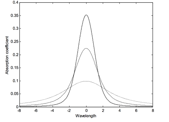
$\text{FIGURE X.4}$

As for the gauss-gauss and lorentz-lorentz profiles, I have appended some details of the integration of the gauss-lorentz profile in the Appendix to this Chapter.

The FWHM or FWHm in wavelength units of a Gaussian profile (i.e. $2g$) is

$$\label{10.5.17}w_G = \frac{\left ( 2kT/m +ξ_\text{m}^2\right )^{\frac{1}{2}}\lambda_0\sqrt{ln 16}}{c}=\frac{1.665 \left ( 2kT/m +ξ_\text{m}^2 \right )^{\frac{1}{2}}\lambda_0}{c}.$$

The FWHM or FWHm in frequency units of a lorentzian profile is

$$\label{10.5.18}w_L = \Gamma /(2\pi)=0.1592 \Gamma ,$$

Here $\Gamma$ is the sum of the radiation damping constant (see section 2) and the contribution from pressure broadening $2 /\overline t$ (see section 6). For the FWHM or FWHm in wavelength units (i.e. $2l$), we have to multiply by $\lambda_0^2 /c$.

Integrating a Voigt Profile

The area under Voigt profile is $2\int_0^\infty V(x)\,dx$, where $V(x)$ is given by Equation $\ref{10.5.14}$, which itself had to be evaluated with a numerical integration. Since the profile is symmetric about $x = 0$, we can integrate from $0\text{ to }\infty$ and multiply by 2. Even so, the double integral might seem like a formidable task. Particularly troublesome would be to integrate a nearly lorentzian profile with extensive wings, because there would then be the problem of how far to go for an upper limit. However, it is not at all a formidable task. The area under the curve given by Equation $\ref{10.5.14}$ is unity! This is easily seen from a physical example. The profile given by Equation $\ref{10.5.14}$ is the convolution of the lorentzian profile of Equation $\ref{10.5.13}$ with the Gaussian profile of Equation $\ref{10.5.12}$, both of which were normalized to unit area. Let us imagine that an emission line is broadened by radiation damping, so that its profile is lorentzian. Now suppose that it is further broadened by thermal broadening (Gaussian profile) to finish as a Voigt profile. (Alternatively, suppose that the line is scanned by a spectrophotometer with a Gaussian sensitivity function.) Clearly, as long as the line is always optically thin, the additional broadening does not affect the integrated intensity.

Now we mentioned in sections 2 and 3 of this chapter that the equivalent width of an absorption line can be calculated from $c \times\text{ central depth }\times$ FWHm, and likewise the area of an emission line is $c \times\text{ height }\times$ FWHM, where $c\text{ is }1.064 ( = \sqrt{\pi / \ln 16} )$ for a Gaussian profile and $1.571 (= \pi/2)$ for a lorentzian profile. We know that the integral of $V(x)$ is unity, and it is a fairly straightforward matter to calculate both the height and the FWHM of $V(x)$. From this, it becomes possible to calculate the constant $c$ as a function of the Gaussian fraction $k_G$. The result of doing this is shown in figure X.4A.

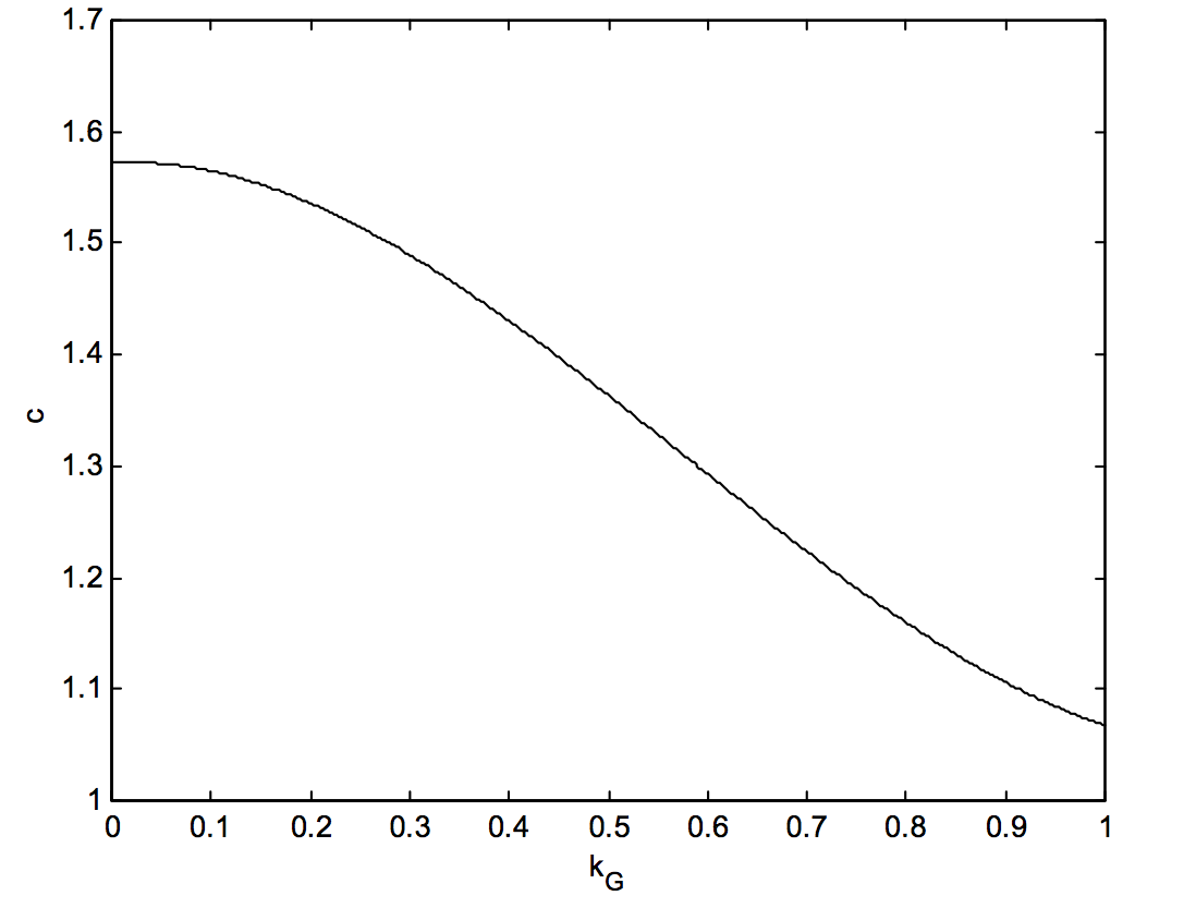
$\text{FIGURE X.4A}$

This curve can be fitted with the empirical Equation

$$\label{10.5.19}c=a_0+a_1k_G+a_2k_G^2+a_3k_G^3,$$

where $a_0 = 1.572,\, a_1 = 0.05288,\, a_2 = -1.323\text{ and }a_3 = 0.7658$. The error incurred in using this formula nowhere exceeds 0.5%; the mean error is 0.25%.

The Voigt Profile in Terms of the Optical Thickness at the Line Center.

Another way to write the Voigt profile that might be useful is

$$\label{10.5.20}\tau (x) = Cl \tau (0) \int_{-\infty}^\infty \frac{\text{exp}[-(ξ-x)^2\ln 2/g^2]}{ξ^2+l^2}\,dξ .$$

Here $x = \lambda - \lambda_0$ and $ξ$ is a dummy variable, which disappears when the definite integral is performed. The Gaussian HWHM is $g=\lambda_0 V_\text{m} \sqrt{\ln 2}/c$, and the lorentzian HWHM is $l=\lambda_0^2 \Gamma /(4\pi c)$. The optical thickness at $\lambda - \lambda_0 = x$ is $\tau (x)$, and the optical thickness at the line centre is $\tau (0)$. $C$ is a dimensionless coefficient, whose value depends on the Gaussian fraction $k_G =g/(g+l)$. $C$ is clearly given by

$$\label{10.5.21}Cl \int_{-\infty}^\infty \frac{\text{exp}[-ξ^2\ln 2/g^2]}{ξ^2+l^2}\,dξ =1.$$

If we now let $l = l^\prime g / \sqrt{\ln 2}$ and $ξ = ξ^\prime g / \sqrt{\ln 2}$, and also make use of the symmetry of the integrand about $ξ = ξ^\prime = 0$, this becomes

$$\label{10.5.22}2Cl^\prime \int_0^\infty \frac{\text{exp}\left ( -ξ^{\prime 2}\right ) }{ξ^{\prime 2}+l^{\prime 2}}dξ^\prime =1.$$

On substitution of $ξ^\prime =\frac{2l^\prime t}{1-t^2}$ (in order to make the limits finite), we obtain

$$\label{10.5.23}4C \int_0^1 \frac{\text{exp}[-\{2l^\prime t/(1-t^2)\}^2 ]}{1+t^2}\,dt =1,$$

which can readily be numerically integrated for a given value of $l^\prime$. Recall that $l/g=1/k_G -1$ and hence that $l^\prime = (1/k_G -1)\sqrt{\ln 2}$. The results of the integration are as follows. The column $C_{\text{approx}}$ is explained following figure X.4B.

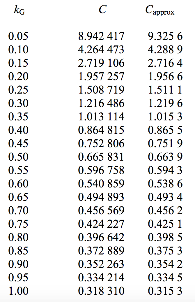
The last entry, the value of $C$ for $k_G = 1$, a pure Gaussian profile, is $1/\pi$. These data are graphed in figure X.4B.

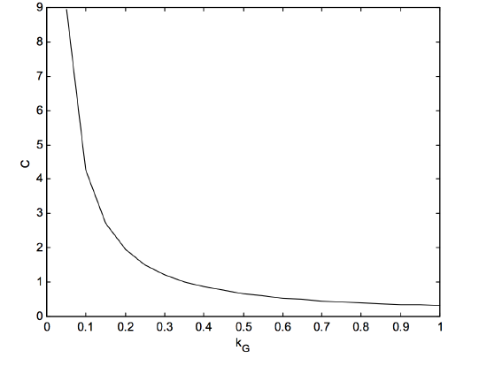
$\text{FIGURE X.4B}$

The empirical formula

$$\label{10.5.24}C_\text{approx}=ak_G^{-b}+c_0+c_1k_G+c_2k_G^2+c_3k_G^3,$$

where

$$\nonumber\begin{align} &a=+0.309031 \quad &&b=+1.132747 \quad &&&c_0=+0.16510 \\ \nonumber&c_1=-0.82999 \quad &&c_2=+1.21782 \quad &&&c_3 =-0.54665 \\ \end{align}$$

fits the curve tolerably well within (but not outside) the range $k_G = 0.15\text{ to }1.00$.