
5.8.6: Rods


- Last updated
- Mar 5, 2022
- Save as PDF

( \newcommand{\kernel}{\mathrm{null}\,}\)
Refer to figure V.5. The potential at P due to the element δx is −Gλδxr=−Gλsecθδθ. The total potential at P is therefore
ψ=−Gλ∫βαsecθdθ=−Gλln[secβ+tanβsecα+tanα].
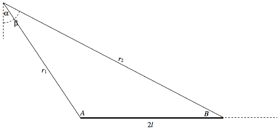
FIGURE V.24
Refer now to figure V.24, in which A=90∘+α and B=90∘−β.
secβ+tanβsecα+tanα=cosα(1+sinβ)cosβ(1+sinα)=sinA(1+cosB)sinB(1−cosA)=2sin12Acos12A.2cos212B2sin12Bcos12B.2sin212A=cot12Acot12B=√s(s−r2)(s−r1)(s−2l)⋅√s(s−r1)(s−2l)(s−r2),
where s=12(r1+r2+2l). (You may want to refer here to the formulas on pp. 37 and 38 of Chapter 2.)
Hence ψ=−Gλln[r1+r2+2lr1+r2−2l].
If r1 and r2 are very large compared with l, they are nearly equal, so let’s put r1+r2=2r and write Equation 5.8.17 as
ψ=−Gm2lln[2r(1+2l2r)2r(1−2l2r)]=−Gm2l[ln(1+lr)−ln(1−lr)].
Maclaurin expand the logarithms, and you will see that, at large distances from the rod, the potential is, expected, −Gm/r.
Let us return to the near vicinity of the rod and to Equation 5.8.16. We see that if we move around the rod in such a manner that we keep r1+r2 constant and equal to 2a, say − that is to say if we move around the rod in an ellipse (see our definition of an ellipse in Chapter 2, Section 2.3) − the potential is constant. In other words the equipotentials are confocal ellipses, with the foci at the ends of the rod. Equation 5.8.16 can be written
ψ=−Gλln(a+la−l).
For a given potential ψ, the equipotential is an ellipse of major axis
2a=2l(eψ/(Gλ)+1eψ/(Gλ)−1),
where 2l is the length of the rod. This knowledge is useful if you are exploring space and you encounter an alien spacecraft or an asteroid in the form of a uniform rod of length 2l.