5.4.7: Solid Cylinder


- Last updated
- Mar 5, 2022
- Save as PDF

( \newcommand{\kernel}{\mathrm{null}\,}\)
We do this not because it has any particular relevance to celestial mechanics, but because it is easy to do. We imagine a solid cylinder, density ρ, radius a, length l. We seek to calculate the field at a point P on the axis, at a distance h from one end of the cylinder (figure V.8).
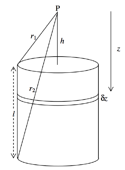
FIGURE V.8
The field at P from an elemental disc of thickness δz a distance z below P is (from Equation 5.4.9)
δg=Gρδzω.
Here ω is the solid angle subtended at P by the disc, which is 2π[1−z(z2+a2)1/2]. Thus the field at P from the entire cylinder is
g=2πGρ∫l+hh[1−z(z2+a2)1/2]dz,
or g=2πGρ(l−√(l+h)2+a2+√h2+a2),
or g=2πGρ(l−r2+r1).
It might also be of interest to express g in terms of the height y(=12l+h) of the point P above the mid-point of the cylinder. Instead of Equation 5.4.21, we then have
g=2πGρ(l−√(y+12l)2+a2+√(y−12l)2+a2).
If the point P is inside the cylinder,at a distance h below the upper end of the cylinder, the limits of integration in Equation 5.4.20 are h and l−h, and the distance y is 12l−h. In terms of y the gravitational field at P is then
g=2πGρ(2y−√(y+12l)2+a2+√(y−12l)2+a2).
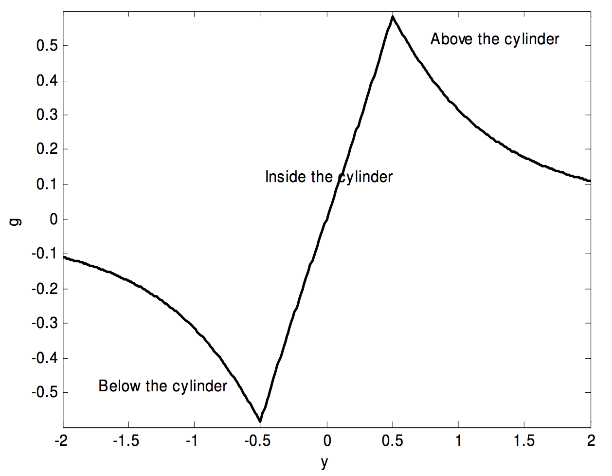
In the graph below I have assumed, by way of example, that l and a are both 1, and I have plotted g in units of 2πGρ (counting g as positive when it is directed downwards) from y=−1 to y=+1. The portion inside the cylinder (−12≤y≤12l), represented by Equation 5.4.24, is almost, but not quite, linear. The field at the centre of the cylinder is, of course, zero.
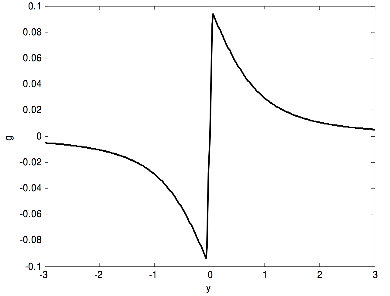
Below, I draw the same graph, but for a thin disc, with a=1 and l=0.1. We see how it is that the field reaches a maximum immediately above or below the disc, but is zero at the centre of the disc.