Search

Text Color

Margin Size

Font Type

Enable Dyslexic Font

Home
Bookshelves
Astronomy & Cosmology
Celestial Mechanics (Tatum)
1: Numerical Methods
1.13: Fitting a Least Squares Polynomial to a Set of Observational Points

1.13: Fitting a Least Squares Polynomial to a Set of Observational Points

Last updated

Mar 5, 2022
Save as PDF
- 1.12: Fitting a Least Squares Straight Line to a Set of Observational Points
- 1.14: Legendre Polynomials

$\newcommand{\vecs}[1]{\overset { \scriptstyle \rightharpoonup} {\mathbf{#1}} }$

$\newcommand{\vecd}[1]{\overset{-\!-\!\rightharpoonup}{\vphantom{a}\smash {#1}}}$

$\newcommand{\id}{\mathrm{id}}$ $\newcommand{\Span}{\mathrm{span}}$

( \newcommand{\kernel}{\mathrm{null}\,}\) $\newcommand{\range}{\mathrm{range}\,}$

$\newcommand{\RealPart}{\mathrm{Re}}$ $\newcommand{\ImaginaryPart}{\mathrm{Im}}$

$\newcommand{\Argument}{\mathrm{Arg}}$ $\newcommand{\norm}[1]{\| #1 \|}$

$\newcommand{\inner}[2]{\langle #1, #2 \rangle}$

$\newcommand{\Span}{\mathrm{span}}$

$\newcommand{\id}{\mathrm{id}}$

$\newcommand{\Span}{\mathrm{span}}$

$\newcommand{\kernel}{\mathrm{null}\,}$

$\newcommand{\range}{\mathrm{range}\,}$

$\newcommand{\RealPart}{\mathrm{Re}}$

$\newcommand{\ImaginaryPart}{\mathrm{Im}}$

$\newcommand{\Argument}{\mathrm{Arg}}$

$\newcommand{\norm}[1]{\| #1 \|}$

$\newcommand{\inner}[2]{\langle #1, #2 \rangle}$

$\newcommand{\Span}{\mathrm{span}}$ $\newcommand{\AA}{\unicode[.8,0]{x212B}}$

$\newcommand{\vectorA}[1]{\vec{#1}} % arrow$

$\newcommand{\vectorAt}[1]{\vec{\text{#1}}} % arrow$

$\newcommand{\vectorB}[1]{\overset { \scriptstyle \rightharpoonup} {\mathbf{#1}} }$

$\newcommand{\vectorC}[1]{\textbf{#1}}$

$\newcommand{\vectorD}[1]{\overrightarrow{#1}}$

$\newcommand{\vectorDt}[1]{\overrightarrow{\text{#1}}}$

$\newcommand{\vectE}[1]{\overset{-\!-\!\rightharpoonup}{\vphantom{a}\smash{\mathbf {#1}}}}$

$\newcommand{\vecs}[1]{\overset { \scriptstyle \rightharpoonup} {\mathbf{#1}} }$

$\newcommand{\vecd}[1]{\overset{-\!-\!\rightharpoonup}{\vphantom{a}\smash {#1}}}$

$\newcommand{\avec}{\mathbf a}$

$\newcommand{\bvec}{\mathbf b}$

$\newcommand{\cvec}{\mathbf c}$

$\newcommand{\dvec}{\mathbf d}$

$\newcommand{\dtil}{\widetilde{\mathbf d}}$

$\newcommand{\evec}{\mathbf e}$

$\newcommand{\fvec}{\mathbf f}$

$\newcommand{\nvec}{\mathbf n}$

$\newcommand{\pvec}{\mathbf p}$

$\newcommand{\qvec}{\mathbf q}$

$\newcommand{\svec}{\mathbf s}$

$\newcommand{\tvec}{\mathbf t}$

$\newcommand{\uvec}{\mathbf u}$

$\newcommand{\vvec}{\mathbf v}$

$\newcommand{\wvec}{\mathbf w}$

$\newcommand{\xvec}{\mathbf x}$

$\newcommand{\yvec}{\mathbf y}$

$\newcommand{\zvec}{\mathbf z}$

$\newcommand{\rvec}{\mathbf r}$

$\newcommand{\mvec}{\mathbf m}$

$\newcommand{\zerovec}{\mathbf 0}$

$\newcommand{\onevec}{\mathbf 1}$

$\newcommand{\real}{\mathbb R}$

$\newcommand{\twovec}[2]{\left[\begin{array}{r}#1 \\ #2 \end{array}\right]}$

$\newcommand{\ctwovec}[2]{\left[\begin{array}{c}#1 \\ #2 \end{array}\right]}$

$\newcommand{\threevec}[3]{\left[\begin{array}{r}#1 \\ #2 \\ #3 \end{array}\right]}$

$\newcommand{\cthreevec}[3]{\left[\begin{array}{c}#1 \\ #2 \\ #3 \end{array}\right]}$

$\newcommand{\fourvec}[4]{\left[\begin{array}{r}#1 \\ #2 \\ #3 \\ #4 \end{array}\right]}$

$\newcommand{\cfourvec}[4]{\left[\begin{array}{c}#1 \\ #2 \\ #3 \\ #4 \end{array}\right]}$

$\newcommand{\fivevec}[5]{\left[\begin{array}{r}#1 \\ #2 \\ #3 \\ #4 \\ #5 \\ \end{array}\right]}$

$\newcommand{\cfivevec}[5]{\left[\begin{array}{c}#1 \\ #2 \\ #3 \\ #4 \\ #5 \\ \end{array}\right]}$

$\newcommand{\mattwo}[4]{\left[\begin{array}{rr}#1 \amp #2 \\ #3 \amp #4 \\ \end{array}\right]}$

$\newcommand{\laspan}[1]{\text{Span}\{#1\}}$

$\newcommand{\bcal}{\cal B}$

$\newcommand{\ccal}{\cal C}$

$\newcommand{\scal}{\cal S}$

$\newcommand{\wcal}{\cal W}$

$\newcommand{\ecal}{\cal E}$

$\newcommand{\coords}[2]{\left\{#1\right\}_{#2}}$

$\newcommand{\gray}[1]{\color{gray}{#1}}$

$\newcommand{\lgray}[1]{\color{lightgray}{#1}}$

$\newcommand{\rank}{\operatorname{rank}}$

$\newcommand{\row}{\text{Row}}$

$\newcommand{\col}{\text{Col}}$

$\renewcommand{\row}{\text{Row}}$

$\newcommand{\nul}{\text{Nul}}$

$\newcommand{\var}{\text{Var}}$

$\newcommand{\corr}{\text{corr}}$

$\newcommand{\len}[1]{\left|#1\right|}$

$\newcommand{\bbar}{\overline{\bvec}}$

$\newcommand{\bhat}{\widehat{\bvec}}$

$\newcommand{\bperp}{\bvec^\perp}$

$\newcommand{\xhat}{\widehat{\xvec}}$

$\newcommand{\vhat}{\widehat{\vvec}}$

$\newcommand{\uhat}{\widehat{\uvec}}$

$\newcommand{\what}{\widehat{\wvec}}$

$\newcommand{\Sighat}{\widehat{\Sigma}}$

$\newcommand{\lt}{<}$

$\newcommand{\gt}{>}$

$\newcommand{\amp}{&}$

$\definecolor{fillinmathshade}{gray}{0.9}$

I shall start by assuming that the values of x are known to a high degree of precision, and all the errors are in the values of $y$ . In other words, I shall calculate a least squares polynomial regression of $y$ upon $x$ . In fact I shall show how to calculate a least squares quadratic regression of $y$ upon $x$ , a quadratic polynomial representing, of course, a parabola. What we want to do is to calculate the coefficients $a_0, \ a_1, \ a_2$ such that the sum of the squares of the residual is least, the residual of the $i$ th point being

$R_i = y_i - (a_0 + a_1 x_i + a_2 x_1^2 ). \label{1.13.1} \tag{1.13.1}$

You have $N$ simultaneous linear Equations of this sort for the three unknowns $a_0, \ a_1$ and $a_2$ . You already know how to find the least squares solution for these, and indeed, after having read Section 1.8, you already have a program for solving the Equations. (Remember that here the unknowns are $a_0, \ a1$ and $a_2$ – not $x$ ! You just have to adjust your notation a bit.) Thus there is no difficulty in finding the least squares quadratic regression of $y$ upon $x$ , and indeed the extension to polynomials of higher degree will now be obvious.

As an Exercise, here are some points that I recently had in a real application:

$\begin{array}{c c} x & y \\ 395.1 & 171.0 \\ 448.1 & 289.0 \\ 517.7 & 399.0 \\ 583.3 & 464.0 \\ 790.2 & 620.0 \\ \end{array}$

Draw these on a sheet of graph paper and draw by hand a nice smooth curve passing as close as possible to the point. Now calculate the least squares parabola (quadratic regression of $y$ upon $x$ ) and see how close you were. I make it $y = -961.34 + 3.7748x - 2.247 \times 10^{-3} x^2$ . It is shown in Figure $\text{I.6C}$ .

I now leave you to work out how to fit a least squares cubic (or indeed any polynomial) regression of $y$ upon $x$ to a set of data points. For the above data, I make the cubic fit to be

$y = -2537.605 + 12.4902x - 0.017777x^2 + 8.89 \times 10^{-6} x^3.$

This is shown in Figure $\text{I.6D}$ , and, on the scale of this drawing it cannot be distinguished (within the range covered by $x$ in the figure) from the quartic Equation that would go exactly through all five points.

The cubic curve is a “better” fit than either the quadratic curve or a straight line in the sense that, the higher the degree of polynomial, the closer the fit and the less the residuals. But higher degree polynomials have more “wiggles”, and you have to ask yourself whether a high-degree polynomial with lots of “wiggles” is really a realistic fit, and maybe you should be satisfied with a quadratic fit. Above all, it is important to understand that it is very dangerous to use the curve that you have calculated to extrapolate beyond the range of $x$ for which you have data – and this is especially true of higher-degree polynomials.

alt
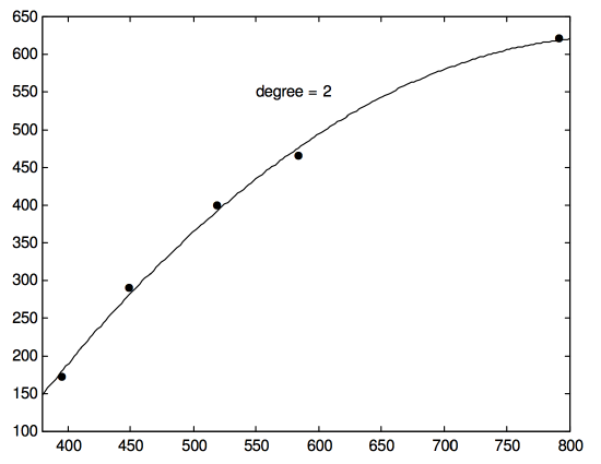
$\text{FIGURE I.6C}$

alt
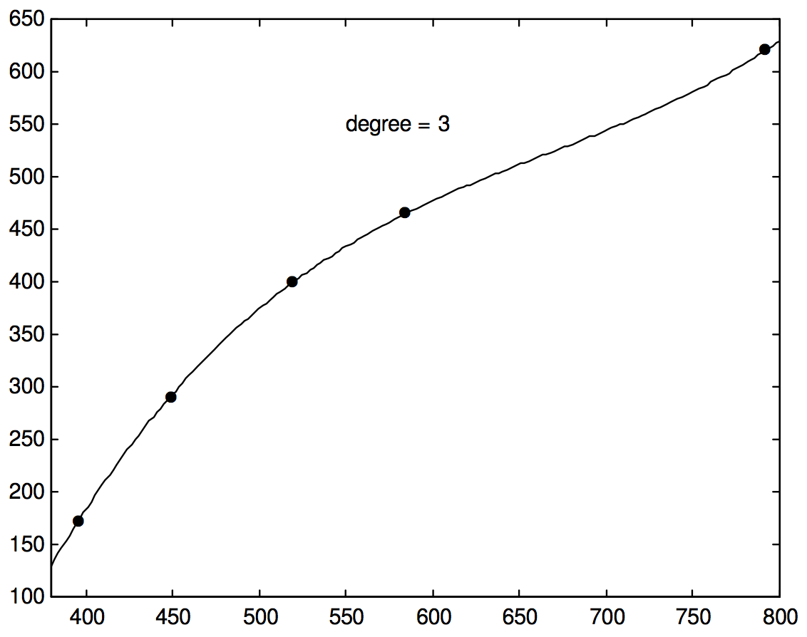
$\text{FIGURE I.6D}$

What happens if the errors in $x$ are not negligible, and the errors in $x$ and $y$ are comparable in size? In that case you want to plot a graph of $y$ against $x$ on a scale such that the unit for $x$ is equal to the standard deviation of the $x$ -residuals from the chosen polynomial and the unit for $y$ is equal to the standard deviation of the $y$ -residuals from the chosen polynomial. For a detailed and thorough account of how to do this, I refer you to a paper by D. York in Canadian Journal of Physics, 44, 1079 (1966).

Support Center

How can we help?