8.7: Worked Examples

Example 8.7 Staircase

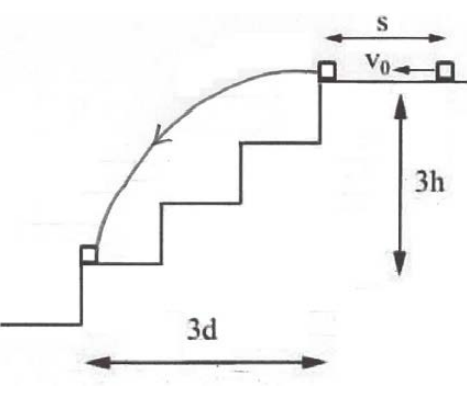
An object of mass m at time t = 0 has speed $v_{0}$ It slides a distance s along a horizontal floor and then off the top of a staircase (Figure 8.35). The coefficient of kinetic friction between the object and the floor is $\mu_{\mathrm{k}}$ The object strikes at the far end of the third stair. Each stair has a rise of h and a run of d . Neglect air resistance and use g for the gravitational constant. (a) What is the distance s that the object slides along the floor?

Figure 8.35 Object falling down a staircase

Solution: There are two distinct stages to the object’s motion, the initial horizontal motion and then free fall. The given final position of the object, at the far end of the third stair, will determine the horizontal component of the velocity at the instant the object left the top of the stairs. This in turn can be used to determine the time the object decelerated along the floor, and hence the distance traveled on the floor. The given quantities are m , v0 , µk , g , h and d.

For the horizontal motion, choose coordinates with the origin at the initial position of the block. Choose the positive $\hat{\mathbf{i}}$ direction to be horizontal, directed to the left in Figure 8.35, $\hat{\mathbf{j}}$-direction to be vertical (up). The forces on the object are gravity $m \overrightarrow{\mathbf{g}}=-m g \hat{\mathbf{j}}$ the normal force $\overrightarrow{\mathbf{N}}=N \hat{\mathbf{j}}$ and the kinetic frictional force $\overrightarrow{\mathbf{f}}_{\mathrm{k}}=-f_{\mathrm{k}} \hat{\mathbf{i}}$. The components of the vectors in Newton’s Second Law, $\overrightarrow{\mathbf{F}}=m \overrightarrow{\mathbf{a}}$, are

$$\begin{aligned} -f_{\mathrm{k}} &=m a_{x} \\ N-m g &=m a_{y} \end{aligned} \nonumber$$

The object does not move in the y -direction; $a_{y}=0$ and thus from the second expression in (8.6.19), $N=m g$ The magnitude of the frictional force is then $f_{\mathrm{k}}=\mu_{\mathrm{k}} N=\mu_{\mathrm{k}} m g$, and the first expression in (8.6.19) gives the x -component of acceleration as $a_{x}=-\mu_{\mathrm{k}} g$ Becasue the acceleration is constant the x -component of the velocity is given by

$$v_{x}(t)=v_{0}+a_{x} t \nonumber$$

where $v_{0}$ is the x -component of the velocity of the object when it just started sliding. The displacement is given by

$$x(t)-x_{0}=v_{0} t+\frac{1}{2} a_{x} t^{2} \nonumber$$

Denote the time the block just leaves the landing by $t_{1}$, where $x\left(t_{1}\right)=s$ and the speed just when it reaches the landing $v_{x}\left(t_{1}\right)=v_{x, 1}$. The initial speed is $v_{0}$ and $x_{0}=0$. Using the initial and final conditions, and the value of the acceleration, Equation (8.6.21) becomes

$$s=v_{0} t_{1}-\frac{1}{2} \mu_{k} g t_{1}^{2} \nonumber$$

Solve Equation (8.6.20) for the time the block reaches the edge of the landing,

$$t_{1}=\frac{v_{x, 1}-v_{0}}{-\mu_{\mathrm{k}} g}=\frac{v_{0}-v_{x, 1}}{\mu_{\mathrm{k}} g} \nonumber$$

Substituting Equation (8.6.23) into Equation (8.6.22) yields

$$s=v_{0}\left(\frac{v_{0}-v_{x, 1}}{\mu_{\mathrm{k}} g}\right)-\frac{1}{2} \mu_{k} g\left(\frac{v_{0}-v_{x, 1}}{\mu_{\mathrm{k}} g}\right)^{2} \nonumber$$

and after some algebra, we can rewrite Equation (8.6.24) as

$$s=\frac{v_{0}^{2}-v_{x, 1}^{2}}{2 \mu_{\mathrm{k}} g} \nonumber$$

From the top of the stair to the far end of the third stair, the object is in free fall. Choose the positive $\hat{\mathbf{i}}$-direction to be horizontal, directed to the left in Figure 8.35, and the positive $\hat{\mathbf{j}}$-direction to be vertical (up) and now choose the origin at the top of the stairs, where the object first goes into free fall. The components of acceleration are $a_{x}=0$, $a_{y}=-g$, the initial x -component of velocity is $v_{x, 1}$, the initial y -component of velocity is $v_{y, 0}=0$, the initial x -position is $x_{0}=0$ and the initial y -position is $y_{0}=0$. Reset $t=0$ when the object just leaves the landing. Let $t_{2}$ denote the instant the object hits the stair, where $y\left(t_{2}\right)=-3 h$ and $x\left(t_{2}\right)=3 d$. The equations describing the object’s position and speed at time $t=t_{2}$ are

$$x\left(t_{2}\right)=3 d=v_{x, 1} t_{2} \nonumber$$

$$y\left(t_{2}\right)=-3 h=-\frac{1}{2} g t_{2}^{2} \nonumber$$

Solve Equation (8.6.26) for $t_{2}$ to yield

$$t_{2}=\frac{3 d}{v_{x, 1}} \nonumber$$

Substitute Equation (8.6.28) into Equation (8.6.27) and eliminate the variable $t_{2}$

$$3 h=\frac{1}{2} g \frac{9 d^{2}}{v_{x, 1}^{2}} \nonumber$$

Equation (8.6.29) can now be solved for the square of the horizontal component of the velocity,

$$v_{x, 1}^{2}=\frac{3 g d^{2}}{2 h} \nonumber$$

Now substitute Equation (8.6.30) into Equation (8.6.25) to determine the distance the object traveled on the landing,

$$s=\frac{v_{0}^{2}-\left(3 g d^{2} / 2 h\right)}{2 \mu_{\mathrm{k}} g} \nonumber$$

Example 8.8 Cart Moving on a Track

Figure 8.36 A falling block will accelerate a cart on a track via the pulling force of the string. The force sensor measures the tension in the string.

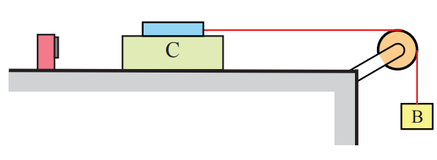
Consider a cart that is free to slide along a horizontal track (Figure 8.36). A force is applied to the cart via a string that is attached to a force sensor mounted on the cart, wrapped around a pulley and attached to a block on the other end. When the block is released the cart will begin to accelerate. The force sensor and cart together have a mass $m_{\mathrm{C}}$, and the suspended block has mass $m_{\mathrm{B}}$. Neglect the small mass of the string and pulley, and assume the string is inextensible. The coefficient of kinetic friction between the cart and the track is $\mu_{\mathrm{k}}$. Determine (i) the acceleration of the cart, and (ii) the tension in the string.

Solution: In general, we would like to draw free-body diagrams on all the individual objects (cart, sensor, pulley, rope, and block) but we can also choose a system consisting of two (or more) objects knowing that the forces of interaction between any two objects will cancel in pairs by Newton’s Third Law. In this example, we shall choose the sensor/cart as one free-body, and the block as the other free-body. The free-body force diagram for the sensor/cart is shown in Figure 8.37.

Figure 8.37 Force diagram on sensor/cart with a vector decomposition of the contact force into horizontal and vertical components

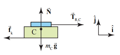
There are three forces acting on the sensor/cart: the gravitational force $m_{\mathrm{C}} \overrightarrow{\mathbf{g}}$, the pulling force $\overrightarrow{\mathbf{T}}_{\mathrm{R}, \mathrm{C}}$ of the rope on the force sensor, and the contact force between the track and the cart. In Figure 8.34, we decompose the contact force into its two components, the kinetic frictional force $\overrightarrow{\mathbf{f}}_{\mathrm{k}}=-f_{\mathrm{k}} \hat{\mathbf{i}}$ and the normal force, $\overrightarrow{\mathbf{N}}=N \hat{\mathbf{j}}$.

The cart is only accelerating in the horizontal direction with $\overrightarrow{\mathbf{a}}_{\mathrm{C}}=a_{\mathrm{C} x} \hat{\mathbf{i}}$ so the component of the force in the vertical direction must be zero, $a_{\mathrm{C}_{y}}=0$. We can now apply Newton’s Second Law in the horizontal and vertical directions and find that

$$\hat{\mathbf{i}}: T_{\mathrm{R}, \mathrm{C}}-f_{\mathrm{k}}=m_{\mathrm{C}} a_{\mathrm{C}, x} \nonumber$$

$$\hat{\mathbf{j}}: \quad N-m_{\mathrm{C}} g=0 \nonumber$$

From Equation (8.6.33), we conclude that the normal component is

$$N=m_{\mathrm{C}} g \nonumber$$

We use Equation (8.6.34) for the normal force to find that the magnitude of the kinetic frictional force is

$$f_{\mathrm{k}}=\mu_{\mathrm{k}} N=\mu_{\mathrm{k}} m_{\mathrm{c}} g \nonumber$$

Then Equation (8.6.32) becomes

$$T_{\mathrm{R}, \mathrm{C}}-\mu_{\mathrm{k}} m_{\mathrm{C}} g=m_{\mathrm{C}} a_{\mathrm{C}, x} \nonumber$$

The force diagram for the block is shown in Figure 8.38. The two forces acting on the block are the pulling force $\overrightarrow{\mathbf{T}}_{\mathrm{R}, \mathrm{B}}$ of the string and the gravitational force $m_{\mathrm{B}} \overrightarrow{\mathbf{g}}$. We now apply Newton’s Second Law to the block and find that

$$\hat{\mathbf{J}}_{\mathrm{B}}: m_{\mathrm{B}} g-T_{\mathrm{R}, \mathrm{B}}=m_{\mathrm{B}} a_{B, y} \nonumber$$

Figure 8.38 Forces acting on the block

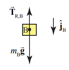
In Equation (8.6.37), the symbol $a_{B, y}$ represents the component of the acceleration with sign determined by our choice of downward direction for the unit vector $\hat{\mathbf{j}}_{\mathrm{B}}$. Note that we made a different choice of direction for the unit vector in the vertical direction in the freebody diagram for the block shown in Figure 8.37. Each free-body diagram has an independent set of unit vectors that define a sign convention for vector decomposition of the forces acting on the free-body and the acceleration of the free-body. In our example, with the unit vector pointing downwards in Figure 8.38, if we solve for the component of the acceleration and it is positive, then we know that the direction of the acceleration is downwards.

There is a second subtle way that signs are introduced with respect to the forces acting on a free-body. In our example, the force between the string and the block acting on the block points upwards, so in the vector decomposition of the forces acting on the block that appears on the left-hand side of Equation (8.6.37), this force has a minus sign and the quantity $\overrightarrow{\mathbf{T}}_{\mathrm{R}, \mathrm{B}}=-T_{\mathrm{R}, \mathrm{B}} \hat{\mathbf{j}}_{\mathrm{B}}$ where $T_{\mathrm{R}, \mathrm{B}}$ is assumed positive.

Our assumption that the mass of the rope and the mass of the pulley are negligible enables us to assert that the tension in the rope is uniform and equal in magnitude to the forces at each end of the rope,

$$T_{\mathrm{R}, \mathrm{B}}=T_{\mathrm{R}, \mathrm{C}} \equiv T \nonumber$$

We also assumed that the string is inextensible (does not stretch). This implies that the rope, block, and sensor/cart all have the same magnitude of acceleration,

$$a_{\mathrm{C}, x}=a_{\mathrm{B}, y} \equiv a \nonumber$$

Using Equations (8.6.38) and (8.6.39), we can now rewrite the equation of motion for the sensor/cart, Equation (8.6.36), as

$$T-\mu_{\mathrm{k}} m_{\mathrm{C}} g=m_{\mathrm{C}} a \nonumber$$

and the equation of motion (8.6.37) for the block as

$$m_{\mathrm{B}} g-T=m_{\mathrm{B}} a \nonumber$$

We have only two unknowns T and a , so we can now solve the two equations (8.6.40) and (8.6.41) simultaneously for the acceleration of the sensor/cart and the tension in the rope. We first solve Equation (8.6.40) for the tension

$$T=\mu_{\mathrm{k}} m_{\mathrm{C}} g+m_{\mathrm{C}} a \nonumber$$

and then substitute Equation (8.6.42) into Equation (8.6.41) and find that

$$m_{\mathrm{B}} g-\left(\mu_{\mathrm{k}} m_{\mathrm{C}} g+m_{\mathrm{C}} a\right)=m_{\mathrm{B}} a \nonumber$$

We can now solve Equation (8.6.43) for the acceleration,

$$a=\frac{m_{\mathrm{B}} g-\mu_{\mathrm{k}} m_{\mathrm{C}} g}{m_{\mathrm{C}}+m_{\mathrm{B}}} \nonumber$$

Substitution of Equation (8.6.44) into Equation (8.6.42) gives the tension in the string,

$$\begin{aligned} T &=\mu_{\mathrm{k}} m_{\mathrm{C}} g+m_{\mathrm{C}} a \\ &=\mu_{\mathrm{k}} m_{\mathrm{C}} g+m_{\mathrm{C}} \frac{m_{\mathrm{B}} g-\mu_{\mathrm{k}} m_{\mathrm{C}} g}{m_{\mathrm{C}}+m_{\mathrm{B}}} \\ &=\left(\mu_{\mathrm{k}}+1\right) \frac{m_{\mathrm{C}} m_{\mathrm{B}}}{m_{\mathrm{C}}+m_{\mathrm{B}}} g \end{aligned} \nonumber$$

In this example, we applied Newton’s Second Law to two objects, one a composite object consisting of the sensor and the cart, and the other the block. We analyzed the forces acting on each object and also any constraints imposed on the acceleration of each object. We used the force laws for kinetic friction and gravitation on each free-body system. The three equations of motion enable us to determine the forces that depend on the parameters in the example: the tension in the rope, the acceleration of the objects, and normal force between the cart and the table.

Example 8.9 Pulleys and Ropes Constraint Conditions

Consider the arrangement of pulleys and blocks shown in Figure 8.39. The pulleys are assumed massless and frictionless and the connecting strings are massless and inextensible. Denote the respective masses of the blocks as $m_{1}$, $m_{2}$, and $m_{3}$. The upper pulley in the figure is free to rotate but its center of mass does not move. Both pulleys have the same radius R . (a) How are the accelerations of the objects related? (b) Draw force diagrams on each moving object. (c) Solve for the accelerations of the objects and the tensions in the ropes.

Figure 8.39 Constrained pulley system

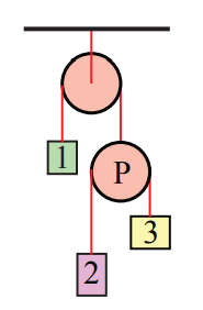
Solution: (a) Choose an origin at the center of the upper pulley. Introduce coordinate functions for the three moving blocks, $y_{1}$, $y_{2}$, and $y_{3}$. Introduce a coordinate function $$\begin{equation}y_{P}\end{equation}$$ for the moving pulley (the pulley on the lower right in Figure 8.40). Choose downward for positive direction; the coordinate system is shown in the figure below then.

Figure 8.40 Coordinated system for pulley system

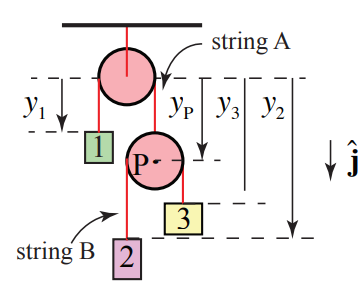
The length of string A is given by

$$l_{A}=y_{1}+y_{P}+\pi R \nonumber$$

where $\pi R$ is the arc length of the rope that is in contact with the pulley. This length is constant, and so the second derivative with respect to time is zero,

$$0=\frac{d^{2} l_{A}}{d t^{2}}=\frac{d^{2} y_{1}}{d t^{2}}+\frac{d^{2} y_{P}}{d t^{2}}=a_{y, 1}+a_{y, P} \nonumber$$

Thus block 1 and the moving pulley’s components of acceleration are equal in magnitude but opposite in sign,

$$a_{y, P}=-a_{y, 1} \nonumber$$

The length of string B is given by

$$l_{B}=\left(y_{3}-y_{p}\right)+\left(y_{2}-y_{p}\right)+\pi R=y_{3}+y_{2}-2 y_{P}+\pi R \nonumber$$

where $\pi R$ is the arc length of the rope that is in contact with the pulley. This length is also constant so the second derivative with respect to time is zero,

$$0=\frac{d^{2} l_{B}}{d t^{2}}=\frac{d^{2} y_{2}}{d t^{2}}+\frac{d^{2} y_{3}}{d t^{2}}-2 \frac{d^{2} y_{p}}{d t^{2}}=a_{y, 2}+a_{y, 3}-2 a_{y, P} \nonumber$$

We can substitute Equation (8.6.48) for the pulley acceleration into Equation (8.6.50) yielding the constraint relation between the components of the acceleration of the three blocks,

$$0=a_{y, 2}+a_{y, 3}+2 a_{y, 1} \nonumber$$

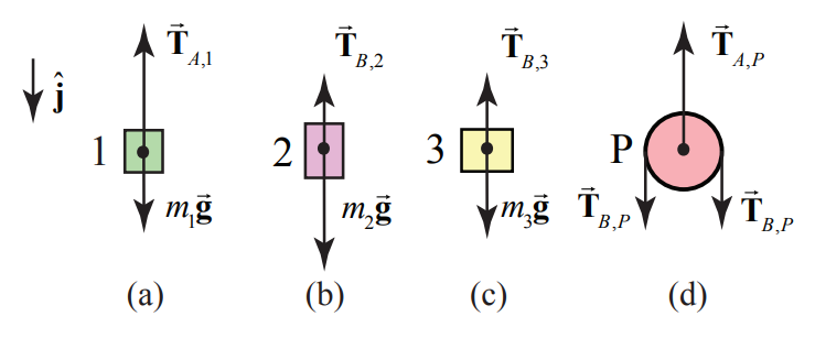
b) Free-body Force diagrams: the forces acting on block 1 are: the gravitational force $m_{1} \overrightarrow{\mathbf{g}}$ and the pulling force $\overrightarrow{\mathbf{T}}_{A, 1}$ of string A acting on the block 1. Denote the magnitude of this force by $T_{A}$ Because the string is assumed to be massless and the pulley is assumed to be massless and frictionless, the tension $T_{A}$ in the string is uniform and equal in magnitude to the pulling force of the string on the block. The free-body diagram on block 1 is shown in Figure 8.41(a).

Figure 8.41 Free-body force diagram on (a) block 1; (b) block 2; (c) block 3; (d) pulley

Newton’s Second Law applied to block 1 is then

$$\hat{\mathbf{j}}: m_{1} g-T_{A}=m_{1} a_{y, 1} \nonumber$$

The forces on the block 2 are the gravitational force $m_{2} \overrightarrow{\mathbf{g}}$ and string B holding the block, $\overrightarrow{\mathbf{T}}_{B, 2}$, with magnitude $T_{B}$. The free-body diagram for the forces acting on block 2 is shown in Figure 8.41(b). Newton’s second Law applied to block 2 is

$$\hat{\mathbf{j}}: m_{2} g-T_{B}=m_{2} a_{y, 2} \nonumber$$

The forces on the block 3 are the gravitational force $m_{3} \overrightarrow{\mathbf{g}}$ and string holding the block, $\overrightarrow{\mathbf{T}}_{B, 3}$, with magnitude equal to $T_{B}$ because pulley P has been assumed to be both frictionless and massless. The free-body diagram for the forces acting on block 3 is shown in Figure 8.41(c). Newton’s second Law applied to block 3 is

$$\hat{\mathbf{j}}: m_{3} g-T_{B}=m_{3} a_{y, 3} \nonumber$$

The forces on the moving pulley P are the gravitational force $m_{P} \overrightarrow{\mathbf{g}}=\overrightarrow{\mathbf{0}}$ (the pulley is assumed massless); string B pulls down on the pulley on each side with a force, $\overrightarrow{\mathbf{T}}_{B, P}$ which has magnitude $T_{B}$. String A holds the pulley up with a force $\overrightarrow{\mathbf{T}}_{A, P}$ with the magnitude $T_{A}$ equal to the tension in string A . The free-body diagram for the forces acting on the moving pulley is shown in Figure 8.41(d). Newton’s second Law applied to the pulley is

$$\hat{\mathbf{j}}: 2 T_{B}-T_{A}=m_{P} a_{y, P}=0 \nonumber$$

Because the pulley is assumed to be massless, we can use this last equation to determine the condition that the tension in the two strings must satisfy,

$$2 T_{B}=T_{A} \nonumber$$

We are now in position to determine the accelerations of the blocks and the tension in the two strings. We record the relevant equations as a summary.

$$0=a_{y, 2}+a_{y, 3}+2 a_{y, 1} \nonumber$$

$$m_{1} g-T_{A}=m_{1} a_{y, 1} \nonumber$$

$$m_{2} g-T_{B}=m_{2} a_{y, 2} \nonumber$$

$$m_{3} g-T_{B}=m_{3} a_{y, 3} \nonumber$$

$$2 T_{B}=T_{A} \nonumber$$

There are five equations with five unknowns, so we can solve this system. We shall first use Equation (8.6.61) to eliminate the tension $T_{A}$ in Equation (8.6.58), yielding

$$m_{1} g-2 T_{B}=m_{1} a_{y, 1} \nonumber$$

We now solve Equations (8.6.59), (8.6.60) and (8.6.62) for the accelerations,

$$a_{y, 2}=g-\frac{T_{B}}{m_{2}} \nonumber$$

$$a_{y, 3}=g-\frac{T_{B}}{m_{3}} \nonumber$$

$$a_{y, 1}=g-\frac{2 T_{B}}{m_{1}} \nonumber$$

We now substitute these results for the accelerations into the constraint equation, Equation (8.6.57),

$$0=g-\frac{T_{B}}{m_{2}}+g-\frac{T_{B}}{m_{3}}+2 g-\frac{4 T_{B}}{m_{1}}=4 g-T_{B}\left(\frac{1}{m_{2}}+\frac{1}{m_{3}}+\frac{4}{m_{1}}\right) \nonumber$$

We can now solve this last equation for the tension in string B ,

$$T_{B}=\frac{4 g}{\left(\frac{1}{m_{2}}+\frac{1}{m_{3}}+\frac{4}{m_{1}}\right)}=\frac{4 g m_{1} m_{2} m_{3}}{m_{1} m_{3}+m_{1} m_{2}+4 m_{2} m_{3}} \nonumber$$

From Equation (8.6.61), the tension in string A is

$$T_{A}=2 T_{B}=\frac{8 g m_{1} m_{2} m_{3}}{m_{1} m_{3}+m_{1} m_{2}+4 m_{2} m_{3}} \nonumber$$

We find the acceleration of block 1 from Equation (8.6.65), using Equation (8.6.67) for the tension in string B,

$$a_{y, 1}=g-\frac{2 T_{B}}{m_{1}}=g-\frac{8 g m_{2} m_{3}}{m_{1} m_{3}+m_{1} m_{2}+4 m_{2} m_{3}}=g \frac{m_{1} m_{3}+m_{1} m_{2}-4 m_{2} m_{3}}{m_{1} m_{3}+m_{1} m_{2}+4 m_{2} m_{3}} \nonumber$$

We find the acceleration of block 2 from Equation (8.6.63), using Equation (8.6.67) for the tension in string B,

$$a_{y, 2}=g-\frac{T_{B}}{m_{2}}=g-\frac{4 g m_{1} m_{3}}{m_{1} m_{3}+m_{1} m_{2}+4 m_{2} m_{3}}=g \frac{-3 m_{1} m_{3}+m_{1} m_{2}+4 m_{2} m_{3}}{m_{1} m_{3}+m_{1} m_{2}+4 m_{2} m_{3}} \nonumber$$

Similarly, we find the acceleration of block 3 from Equation (8.6.64), using Equation (8.6.67) for the tension in string B,

$$a_{y, 3}=g-\frac{T_{B}}{m_{3}}=g-\frac{4 g m_{1} m_{2}}{m_{1} m_{3}+m_{1} m_{2}+4 m_{2} m_{3}}=g \frac{m_{1} m_{3}-3 m_{1} m_{2}+4 m_{2} m_{3}}{m_{1} m_{3}+m_{1} m_{2}+4 m_{2} m_{3}} \nonumber$$

As a check on our algebra we note that

$$\begin{array}{l} 2 a_{1, y}+a_{2, y}+a_{3, y}= \\ 2 g \frac{m_{1} m_{3}+m_{1} m_{2}-4 m_{2} m_{3}}{m_{1} m_{3}+m_{1} m_{2}+4 m_{2} m_{3}}+g \frac{-3 m_{1} m_{3}+m_{1} m_{2}+4 m_{2} m_{3}}{m_{1} m_{3}+m_{1} m_{2}+4 m_{2} m_{3}}+g \frac{m_{1} m_{3}-3 m_{1} m_{2}+4 m_{2} m_{3}}{m_{1} m_{3}+m_{1} m_{2}+4 m_{2} m_{3}} \\ =0 \end{array} \nonumber$$

Example 8.10 Accelerating Wedge

Figure 8.42 Block on accelerating wedge

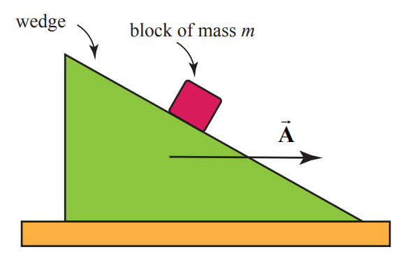
A 45o wedge is pushed along a table with constant acceleration $\overrightarrow{\mathbf{A}}$ according to an observer at rest with respect to the table. A block of mass m slides without friction down the wedge (Figure 8.42). Find its acceleration with respect to an observer at rest with respect to the table. Write down a plan for finding the magnitude of the acceleration of the block. Make sure you clearly state which concepts you plan to use to calculate any relevant physical quantities. Also clearly state any assumptions you make. Be sure you include any free-body force diagrams or sketches that you plan to use.

Solution: Choose a coordinate system for the block and wedge as shown in Figure 8.43. Then $\overrightarrow{\mathbf{A}}=A_{x, w} \hat{\mathbf{i}}$ where $A_{x, w}$ is the x-component of the acceleration of the wedge.

Figure 8.43 Coordinate system for block on accelerating wedge

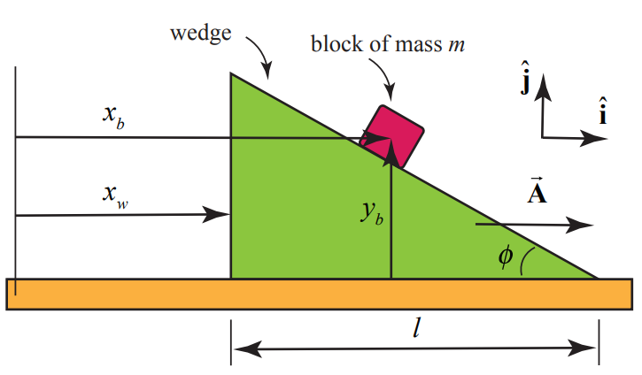
We shall apply Newton’s Second Law to the block sliding down the wedge. Because the wedge is accelerating, there is a constraint relation between the x - and y - components of the acceleration of the block. In order to find that constraint we choose a coordinate system for the wedge and block sliding down the wedge shown in the figure below. We shall find the constraint relationship between the components of the accelerations of the block and wedge by a geometric argument. From the figure above, we see that

$$\tan \phi=\frac{y_{b}}{l-\left(x_{b}-x_{w}\right)} \nonumber$$

Therefore

$$y_{b}=\left(l-\left(x_{b}-x_{w}\right)\right) \tan \phi \nonumber$$

If we differentiate Equation (8.6.73) twice with respect to time noting that

$$\frac{d^{2} l}{d t^{2}}=0 \nonumber$$

we have that

$$\frac{d^{2} y_{b}}{d t^{2}}=-\left(\frac{d^{2} x_{b}}{d t^{2}}-\frac{d^{2} x_{w}}{d t^{2}}\right) \tan \phi \nonumber$$

Therefore

$$a_{b, y}=-\left(a_{b, x}-A_{x, w}\right) \tan \phi \nonumber$$

where

$$A_{x, w}=\frac{d^{2} x_{w}}{d t^{2}} \nonumber$$

We now draw a free-body force diagram for the block (Figure 8.44). Newton’s Second Law in the $\hat{\mathbf{i}}$ - direction becomes

$$N \sin \phi=m a_{b x} \nonumber$$

and the $\hat{\mathbf{j}}$-direction becomes

$$N \cos \phi-m g=m a_{b, y} \nonumber$$

Figure 8.44 Free-body force diagram on block

We can solve for the normal force from Equation (8.6.78):

$$N=\frac{m a_{b, x}}{\sin \phi} \nonumber$$

We now substitute Equation (8.6.76) and Equation (8.6.80) into Equation (8.6.79) yielding

$$\frac{m a_{b, x}}{\sin \phi} \cos \phi-m g=m\left(-\left(a_{b, x}-A_{w, x}\right) \tan \phi\right) \nonumber$$

We now clean this up yielding

$$m a_{b, x}(\operatorname{cotan} \phi+\tan \phi)=m\left(g+A_{w, x} \tan \phi\right) \nonumber$$

Thus the x-component of the acceleration is then

$$a_{b, x}=\frac{g+A_{w, x} \tan \phi}{\operatorname{cotan} \phi+\tan \phi} \nonumber$$

From Equation (8.6.76), the y -component of the acceleration is then

$$a_{b, y}=-\left(a_{b, x}-A_{w, x}\right) \tan \phi=-\left(\frac{g+A_{w, x} \tan \phi}{\operatorname{cotan} \phi+\tan \phi}-A_{w, x}\right) \tan \phi \nonumber$$

This simplifies to

$$a_{b, y}=\frac{A_{w, x}-g \tan \phi}{\operatorname{cotan} \phi+\tan \phi} \nonumber$$

When $\phi=45^{\circ}$, cotan $45^{\circ}=\tan 45^{\circ}=1$, and so Equation (8.6.83) becomes

$$a_{b, x}=\frac{g+A_{w, x}}{2} \nonumber$$

and Equation (8.6.85) becomes

$$a_{b, y}=\frac{A-g}{2} \nonumber$$

The magnitude of the acceleration is then

$$\begin{aligned} a=\sqrt{a_{b, x}^{2}+a_{b, y}^{2}} &=\sqrt{\left(\frac{g+A_{w x}}{2}\right)^{2}+\left(\frac{A_{w x}-g}{2}\right)^{2}} \\ a &=\sqrt{\left(\frac{g^{2}+A_{w}^{2}}{2}\right)} \end{aligned} \nonumber$$

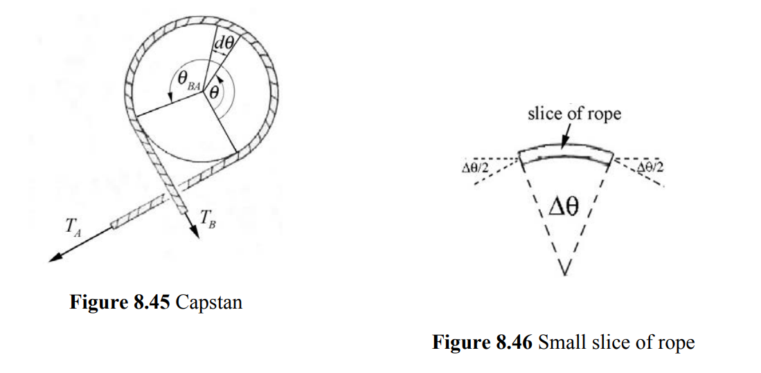
Example 8.11: Capstan

A device called a capstan is used aboard ships in order to control a rope that is under great tension. The rope is wrapped around a fixed drum of radius R , usually for several turns (Figure 8.45 shows about three fourths turn as seen from overhead). The load on the rope pulls it with a force $T_{A}$ and the sailor holds the other end of the rope with a much smaller force $T_{B}$. The coefficient of static friction between the rope and the drum is $\mu_{\mathrm{s}}$. The sailor is holding the rope so that it is just about to slip. Show that $T_{B}=T_{A} e^{-\mu_{s} \theta_{B A}}$ where $\theta_{B A}$ is the angle subtended by the rope on the drum.

Figure 8.47. The right edge of the slice is at angle θ and the left edge of the slice is at $\theta+\Delta \theta$ The angle edge end of the slice makes with the horizontal is $\Delta \theta / 2$. There are four forces acting on this section of the rope. The forces are the normal force between the capstan and the rope pointing outward, a static frictional force and the tensions at either end of the slice. The rope is held at the just slipping point, so if the load exerts a greater force the rope will slip to the right. Therefore the direction of the static frictional force between the capstan and the rope, acting on the rope, points to the left. The tension on the right side of the slice is denoted by $T(\theta) \equiv T$, while the tension on the left side of the slice is denoted by $T(\theta+\Delta \theta) \equiv T+\Delta T$. Does the tension in this slice from the right side to the left, increase, remain the same, or decrease? The tension decreases because the load on the left side is less than the load on the right side. Note that $\Delta T<0$.

Figure 8.47 Free-body force diagram on small slice of rope

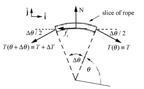
The vector decomposition of the forces is given by

$$\hat{\mathbf{i}}: T \cos (\Delta \theta / 2)-f_{s}-(T+\Delta T) \cos (\Delta \theta / 2) \nonumber$$

$$\hat{\mathbf{j}}:-T \sin (\Delta \theta / 2)+N-(T+\Delta T) \sin (\Delta \theta / 2) \nonumber$$

For small angles $\Delta \theta$, $\cos (\Delta \theta / 2) \cong 1$, and $\sin (\Delta \theta / 2) \cong \Delta \theta / 2$ Using the small angle approximations, the vector decomposition of the forces in the x -direction (the $\hat{\mathbf{i}}$ direction) becomes

$$\begin{aligned} T \cos (\Delta \theta / 2)-f_{s}-(T+\Delta T) \cos (\Delta \theta / 2) & \simeq T-f_{s}-(T+\Delta T) \\ &=-f_{s}-\Delta T \end{aligned} \nonumber$$

By the static equilibrium condition the sum of the x -components of the forces is zero,

$$-f_{\mathrm{s}}-\Delta T=0 \nonumber$$

The vector decomposition of the forces in the y -direction (the $+\hat{\mathbf{j}}$-direction) is approximately

$$\begin{aligned} -T \sin (\Delta \theta / 2)+N-(T+\Delta T) \sin (\Delta \theta / 2) & \simeq-T \Delta \theta / 2+N-(T+\Delta T) \Delta \theta / 2 \\ &=-T \Delta \theta+N-\Delta T \Delta \theta / 2 \end{aligned} \nonumber$$

In the last equation above we can ignore the terms proportional to $\Delta T \Delta \theta$ because these are the product of two small quantities and hence are much smaller than the terms proportional to either $\Delta T$ or $\Delta \theta$. The vector decomposition in the y -direction becomes

$$-T \Delta \theta+N \nonumber$$

Static equilibrium implies that this sum of the y -components of the forces is zero,

$$-T \Delta \theta+N=0 \nonumber$$

We can solve this equation for the magnitude of the normal force

$$N=T \Delta \theta \nonumber$$

The just slipping condition is that the magnitude of the static friction attains its maximum value

$$f_{\mathrm{s}}=\left(f_{\mathrm{s}}\right)_{\max }=\mu_{\mathrm{s}} N \nonumber$$

We can now combine the Equations (8.6.92) and (8.6.97) to yield

$$\Delta T=-\mu_{s} N \nonumber$$

Now substitute the magnitude of the normal force, Equation (8.6.96), into Equation (8.6.98), yielding

$$-\mu_{s} T \Delta \theta-\Delta T=0 \nonumber$$

Finally, solve this equation for the ratio of the change in tension to the change in angle,

$$\frac{\Delta T}{\Delta \theta}=-\mu_{\mathrm{s}} T \nonumber$$

The derivative of tension with respect to the angle θ is defined to be the limit

$$\frac{d T}{d \theta} \equiv \lim _{\Delta \theta \rightarrow 0} \frac{\Delta T}{\Delta \theta} \nonumber$$

and Equation (8.6.100) becomes

$$\frac{d T}{d \theta}=-\mu_{s} T \nonumber$$

This is an example of a first order linear differential equation that shows that the rate of change of tension with respect to the angle θ is proportional to the negative of the tension at that angle θ . This equation can be solved by integration using the technique of separation of variables. We first rewrite Equation (8.6.102) as

$$\frac{d T}{T}=-\mu_{s} d \theta \nonumber$$

Integrate both sides, noting that when θ = 0 , the tension is equal to force of the load $T_{A}$ and when angle $\theta=\theta_{A, B}$ the tension is equal to the force $T_{B}$ the sailor applies to the rope,

$$\int_{T=T_{A}}^{T=T_{B}} \frac{d T}{T}=-\int_{\theta=0}^{\theta=\theta_{B A}} \mu_{s} d \theta \nonumber$$

The result of the integration is

$$\ln \left(\frac{T_{B}}{T_{A}}\right)=-\mu_{s} \theta_{B A} \nonumber$$

Note that the exponential of the natural logarithm

$$\exp \left(\ln \left(\frac{T_{B}}{T_{A}}\right)\right)=\frac{T_{B}}{T_{A}} \nonumber$$

so exponentiating both sides of Equation (8.6.105) yields

$$\frac{T_{B}}{T_{A}}=e^{-\mu_{\mathrm{s}} \theta_{B A}} \nonumber$$

the tension decreases exponentially,

$$T_{B}=T_{A} e^{-\mu_{s} \theta_{B A}} \nonumber$$

Because the tension decreases exponentially, the sailor need only apply a small force to prevent the rope from slipping.

Example 8.12 Free Fall with Air Drag

Consider an object of mass m that is in free fall but experiencing air resistance. The magnitude of the drag force is given by Equation (8.6.1), where $\rho$ is the density of air, A is the cross-sectional area of the object in a plane perpendicular to the motion, and $C_{D}$ the drag coefficient. Assume that the object is released from rest and very quickly attains speeds in which Equation (8.6.1) applies. Determine (i) the terminal velocity, and (ii) the velocity of the object as a function of time.

Solution: Choose positive y -direction downwards with the origin at the initial position of the object as shown in Figure 8.48(a).

Figure 8.48 (a) Coordinate system for marble; (b) free body force diagram on marble

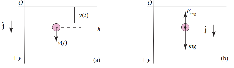
There are two forces acting on the object: the gravitational force, and the drag force which is given by Equation (8.6.1). The free body diagram is shown in the Figure 8.48(b). Newton’s Second Law is then

$$m g-(1 / 2) C_{D} A \rho v^{2}=m \frac{d v}{d t} \nonumber$$

Set $\beta=(1 / 2) C_{D} A \rho$. Newton’s Second Law can then be written as

$$m g-\beta v^{2}=m \frac{d v}{d t} \nonumber$$

Initially when the object is just released with v = 0 , the air drag is zero and the acceleration dv / dt is maximum. As the object increases its velocity, the air drag becomes larger and dv / dt decreases until the object reaches terminal velocity and dv / dt = 0 . Set dv / dt = 0 in Equation (8.6.15) and solve for the terminal velocity yielding.

$$v_{\infty}=\sqrt{\frac{m g}{\beta}}=\sqrt{\frac{2 m g}{C_{D} A \rho}} \nonumber$$

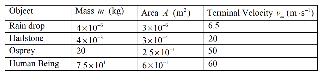
Values for the magnitude of the terminal velocity is shown in Table 8.3 for a variety of objects with the same drag coefficient $C_{D}=0.5$

Table 8.3 Terminal Velocities for Different Sized Objects with $C_{D}=0.5$

In order to integrate Equation (8.6.15), we shall apply the technique of separation of variables and integration by partial fractions. First rewrite Equation (8.6.15) as

$$\frac{-\beta}{m} d t=\frac{d v}{\left(v^{2}-\frac{m g}{\beta}\right)}=\frac{d v}{\left(v^{2}-v_{\infty}^{2}\right)}=\left(-\frac{1}{2 v_{\infty}\left(v+v_{\infty}\right)}+\frac{1}{2 v_{\infty}\left(v-v_{\infty}\right)}\right) d v \nonumber$$

An integral expression of Equation (8.6.112) is then

$$-\int_{v^{\prime}=0}^{v^{\prime}=v(t)} \frac{d v^{\prime}}{2 v_{\infty}\left(v^{\prime}+v_{\infty}\right)}+\int_{v=0}^{v=v(t)} \frac{d v^{\prime}}{2 v_{\infty}\left(v^{\prime}-v_{\infty}\right)}=-\frac{\beta}{m} \int_{t=0}^{t^{\prime}=t} d t^{\prime} \nonumber$$

Integration yields

$$\begin{array}{l} -\int_{v^{\prime}=0}^{v^{\prime}=v(t)} \frac{d v^{\prime}}{2 v_{\infty}\left(v^{\prime}+v_{\infty}\right)}+\int_{v^{\prime}=0}^{v^{\prime}=v(t)} \frac{d v^{\prime}}{2 v_{\infty}\left(v^{\prime}-v_{\infty}\right)}=-\frac{\beta^{t^{\prime}=t}}{m} \int_{t^{\prime}=0}^{t} d t^{\prime} \\ \frac{1}{2 v_{\infty}}\left(-\ln \left(\frac{v(t)+v_{\infty}}{v_{\infty}}\right)+\ln \left(\frac{v_{\infty}-v(t)}{v_{\infty}}\right)\right)=-\frac{\beta}{m} t \end{array} \nonumber$$

After some algebraic manipulations, Equation (8.6.114) can be rewritten as

$$\ln \left(\frac{v_{\infty}-v(t)}{v(t)+v_{\infty}}\right)=-\frac{2 v_{\infty} \beta}{m} t \nonumber$$

Exponentiate Equation (8.6.115) yields

$$\left(\frac{v_{\infty}-v(t)}{v(t)+v_{\infty}}\right)=e^{-\frac{2 v_{\omega} \beta}{m} t} \nonumber$$

After some algebraic rearrangement the y -component of the velocity as a function of time is given by

$$\begin{array}{c} v(t)=v_{\infty}\left(\frac{1-e^{-\frac{2 v_{w} \beta_{t}}{m}}}{1+e^{-\frac{2 v_{\infty} \beta_{t}}{m}}}\right)=v_{\infty} \tan h\left(\frac{v_{\infty} \beta}{m} t\right) \\ \text { where } \frac{v_{\infty} \beta}{m}=\frac{\beta}{m} \sqrt{\frac{m g}{\beta}}=\sqrt{\frac{\beta g}{m}}=\sqrt{\frac{(1 / 2) C_{D} A \rho g}{m}} \end{array} \nonumber$$