2.1: Lagrange Equation

In many cases, the constraints imposed on the 3D motion of a system of $N$ particles may be described by $N$ vector (i.e. $3 N$ scalar) algebraic equations $$\mathbf{r}_{k}=\mathbf{r}_{k}\left(q_{1}, q_{2}, \ldots, q_{j}, \ldots, q_{J}, t\right), \quad \text { with } 1 \leq k \leq N,$$ where $q_{j}$ are certain generalized coordinates that (together with constraints) completely define the system position. Their number $J \leq 3 N$ is called the number of the actual degrees of freedom of the system. The constraints that allow such description are called holonomic. ${ }^{1}$

For example, for the problem discussed briefly in Section 1.5, namely the bead sliding along a rotating ring (Figure 1), $J=1$, because with the constraints imposed by the ring, the bead’s position is uniquely determined by just one generalized coordinate - for example, its polar angle $\theta$.

Figure 2.1. A bead on a rotating ring as an example of a system with just one degree of freedom $(J=1)$.

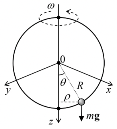
Indeed, selecting the reference frame as shown in Figure 1 and using the well-known formulas for the spherical coordinates, ${ }^{2}$ we see that in this case, Eq. (1) has the form $$\mathbf{r} \equiv\{x, y, z\}=\{R \sin \theta \cos \varphi, R \sin \theta \sin \varphi, R \cos \theta\}, \quad \text { where } \varphi=\omega t+\text { const },$$ with the last constant depending on the exact selection of the axes $x$ and $y$ and the time origin. Since the angle $\varphi$, in this case, is a fixed function of time, and $R$ is a fixed constant, the particle’s position in space at any instant $t$ is completely determined by the value of its only generalized coordinate $\theta$. (Note that its dimensionality is different from that of Cartesian coordinates!)

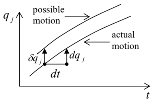
Now returning to the general case of $J$ degrees of freedom, let us consider a set of small variations (alternatively called "virtual displacements") $\delta q_{j}$ allowed by the constraints. Virtual displacements differ from the actual small displacements (described by differentials $d q_{j}$ proportional to time variation $d t$ ) in that $\delta q_{j}$ describes not the system’s motion as such, but rather its possible variation see Figure 1 .

Figure 2.2. Actual displacement $d q_{j}$ vs. the virtual one (i.e. variation) $\delta q_{j}$.

Generally, operations with variations are the subject of a special field of mathematics, the calculus of variations. ${ }^{3}$ However, the only math background necessary for our current purposes is the understanding that operations with variations are similar to those with the usual differentials, though we need to watch carefully what each variable is a function of. For example, if we consider the variation of the radius vectors (1), at a fixed time $t$, as a function of independent variations $\delta q_{j}$, we may use the usual formula for the differentiation of a function of several arguments: ${ }^{4}$ $$\delta \mathbf{r}_{k}=\sum_{j} \frac{\partial \mathbf{r}_{k}}{\partial q_{j}} \delta q_{j} .$$ Now let us break the force acting upon the $k^{\text {th }}$ particle into two parts: the frictionless, constraining part $\mathbf{N}_{k}$ of the reaction force and the remaining part $\mathbf{F}_{k}$ - including the forces from other sources and possibly the friction part of the reaction force. Then the $2^{\text {nd }}$ Newton law for the $k^{\text {th }}$ particle of the system may be rewritten as $$m_{k} \dot{\mathbf{v}}_{k}-\mathbf{F}_{k}=\mathbf{N}_{k} .$$ Since any variation of the motion has to be allowed by the constraints, its $3 N$-dimensional vector with $N$ $3 \mathrm{D}$-vector components $\delta \mathbf{r}_{k}$ has to be perpendicular to the $3 N$-dimensional vector of the constraining forces, also with $N$ 3D-vector components $\mathbf{N}_{k}$. (For example, for the problem shown in Figure 2.1, the virtual displacement vector $\delta \mathbf{r}_{k}$ may be directed only along the ring, while the constraining force $\mathbf{N}$, exerted by the ring, has to be perpendicular to that direction.) This condition may be expressed as $$\sum_{k} \mathbf{N}_{k} \cdot \delta \mathbf{r}_{k}=0$$ where the scalar product of $3 N$-dimensional vectors is defined exactly like that of $3 \mathrm{D}$ vectors, i.e. as the sum of the products of the corresponding components of the operands. The substitution of Eq. (4) into Eq. (5) results in the so-called $D$ ’Alembert principle: $^{5}$ $$\sum_{k}\left(m_{k} \dot{\mathbf{v}}_{k}-\mathbf{F}_{k}\right) \cdot \delta \mathbf{r}_{k}=0$$ Now we may plug Eq. (3) into Eq. (6) to get $$\sum_{j}\left\{\sum_{k} m_{k} \dot{\mathbf{v}}_{k} \cdot \frac{\partial \mathbf{r}_{k}}{\partial q_{j}}-\mathscr{F}_{j}\right\} \delta q_{j}=0,$$ where the scalars $\mathscr{J}_{j}$, called the generalized forces, are defined as follows: ${ }^{6}$

Generalized force

$$\ \mathscr{F}_{j} \equiv \sum_{k} \mathbf{F}_{k} \cdot \frac{\partial \mathbf{r}_{k}}{\partial q_{j}}.$$

Now we may use the standard argument of the calculus of variations: for the left-hand side of Eq. (7) to be zero for an arbitrary selection of independent variations $\ \delta q_{j}$, the expressions in the curly brackets, for every $\ j$, should equal zero. This gives us the desired set of $\ J \leq 3 N$ equations

$$\ \sum_{k} m_{k} \dot{\mathbf{v}}_{k} \cdot \frac{\partial \mathbf{r}_{k}}{\partial q_{j}}-\mathscr{F}_{j}=0;$$

what remains is just to recast them in a more convenient form.

First, using the differentiation by parts to calculate the following time derivative: $$\frac{d}{d t}\left(\mathbf{v}_{k} \cdot \frac{\partial \mathbf{r}_{k}}{\partial q_{j}}\right)=\dot{\mathbf{v}}_{k} \cdot \frac{\partial \mathbf{r}_{k}}{\partial q_{j}}+\mathbf{v}_{k} \cdot \frac{d}{d t}\left(\frac{\partial \mathbf{r}_{k}}{\partial q_{j}}\right),$$ we may notice that the first term on the right-hand side is exactly the scalar product in the first term of Eq. (9).

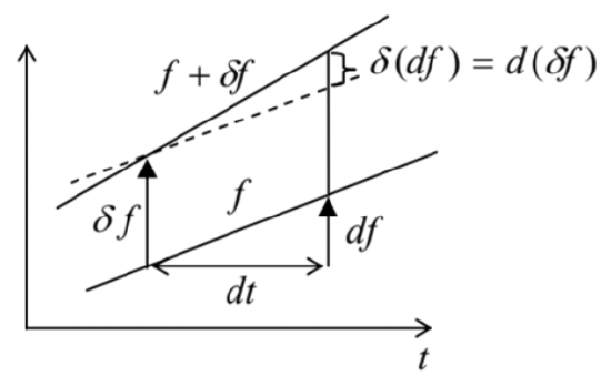
Second, let us use another key fact of the calculus of variations (which is, essentially, evident from Figure 3): the differentiation of a variable over time and over the generalized coordinate variation (at a fixed time) are interchangeable operations. As a result, in the second term on the right-hand side of Eq. (10) we may write $$\frac{d}{d t}\left(\frac{\partial \mathbf{r}_{k}}{\partial q_{j}}\right)=\frac{\partial}{\partial q_{j}}\left(\frac{d \mathbf{r}_{k}}{d t}\right) \equiv \frac{\partial \mathbf{v}_{k}}{\partial q_{j}}$$

Figure 2.3. The variation of the differential (of any smooth function $f$ ) is equal to the differential of its variation.

Finally, let us differentiate Eq. (1) over time: $$\mathbf{v}_{k} \equiv \frac{d \mathbf{r}_{k}}{d t}=\sum_{j} \frac{\partial \mathbf{r}_{k}}{\partial q_{j}} \dot{q}_{j}+\frac{\partial \mathbf{r}_{k}}{\partial t} .$$ This equation shows that particle velocities $\mathbf{v}_{k}$ may be considered to be linear functions of the generalized velocities $\dot{q}_{j}$ considered as independent variables, with proportionality coefficients $$\frac{\partial \mathbf{v}_{k}}{\partial \dot{q}_{j}}=\frac{\partial \mathbf{r}_{k}}{\partial q_{j}} .$$ With the account of Eqs. (10), (11), and (13), Eq. (9) turns into $$\frac{d}{d t} \sum_{k} m_{k} \mathbf{v}_{k} \cdot \frac{\partial \mathbf{v}_{k}}{\partial \dot{q}_{j}}-\sum_{k} m_{k} \mathbf{v}_{k} \cdot \frac{\partial \mathbf{v}_{k}}{\partial q_{j}}-\mathscr{F}_{j}=0$$ This result may be further simplified by making, for the total kinetic energy of the system, $$T \equiv \sum_{k} \frac{m_{k}}{2} v_{k}^{2}=\frac{1}{2} \sum_{k} m_{k} \mathbf{v}_{k} \cdot \mathbf{v}_{k},$$ the same commitment as for $\mathbf{v}_{k}$, i.e. considering $T$ a function of not only the generalized coordinates $q_{j}$ and time $t$ but also of the generalized velocities $\dot{q}_{i}-$ as variables independent of $q_{j}$ and $t$. Then we may calculate the partial derivatives of $T$ as $$\frac{\partial T}{\partial q_{j}}=\sum_{k} m_{k} \mathbf{v}_{k} \cdot \frac{\partial \mathbf{v}_{k}}{\partial q_{j}}, \quad \frac{\partial T}{\partial \dot{q}_{j}}=\sum_{k} m_{k} \mathbf{v}_{k} \cdot \frac{\partial \mathbf{v}_{k}}{\partial \dot{q}_{j}}$$ and notice that they are exactly the two sums participating in Eq. (14). As a result, we get a system of $J$ Lagrange equations, ${ }^{7}$ $$\frac{d}{d t} \frac{\partial T}{\partial \dot{q}_{j}}-\frac{\partial T}{\partial q_{j}}-\mathscr{F}_{j}=0, \quad \text { for } j=1,2, \ldots, J$$ Their big advantage over the initial Newton law equations (4) is that the Lagrange equations do not include the constraining forces $\mathbf{N}_{k}$, and thus there are only $J$ of them - typically much fewer than $3 N$.

This is as far as we can go for arbitrary forces. However, if all the forces may be expressed in the form similar to, but somewhat more general than Eq. (1.22), $\mathbf{F}_{k}=-\nabla_{k} U\left(\mathbf{r}_{1}, \mathbf{r}_{2}, \ldots, \mathbf{r}_{N}, t\right)$, where $U$ is the effective potential energy of the system, ${ }^{8}$ and $\nabla_{k}$ denotes the spatial differentiation over coordinates of the $k^{\text {th }}$ particle, we may recast Eq. (8) into a simpler form: $$\mathscr{T}_{j} \equiv \sum_{k} \mathbf{F}_{k} \cdot \frac{\partial \mathbf{r}_{k}}{\partial q_{j}}=-\sum_{k}\left(\frac{\partial U}{\partial x_{k}} \frac{\partial x_{k}}{\partial q_{j}}+\frac{\partial U}{\partial y_{k}} \frac{\partial y_{k}}{\partial q_{j}}+\frac{\partial U}{\partial z_{i}} \frac{\partial z_{i}}{\partial q_{j}}\right) \equiv-\frac{\partial U}{\partial q_{j}} .$$ Since we assume that $U$ depends only on particle coordinates (and possibly time), but not velocities: $\partial U / \partial \dot{q}_{j}=0$, with the substitution of Eq. (18), the Lagrange equation (17) may be represented in the socalled canonical form: $$\frac{d}{d t} \frac{\partial L}{\partial \dot{q}_{j}}-\frac{\partial L}{\partial q_{j}}=0,$$ where $L$ is the Lagrangian function (sometimes called just the "Lagrangian"), defined as $$L \equiv T-U \text {. }$$ (It is crucial to distinguish this function from the mechanical energy $(1.26), E=T+U$.)

Note also that according to Eq. (2.18), for a system under the effect of an additional generalized external force $\mathscr{T}_{j}(t)$ we have to use, in all these relations, not the internal potential energy $U^{\text {(int) }}$ of the system, but its Gibbs potential energy $U \equiv U^{(\text {int })}-\mathscr{J}_{j} q_{j}-$ see the discussion in Sec. 1.4.

Using the Lagrangian approach in practice, the reader should always remember that, first, each system has only one Lagrange function (19b), but is described by $J \geq 1$ Lagrange equations (19a), with $j$ taking values $1,2, \ldots, J$, and second, that differentiating the function $L$, we have to consider the generalized velocities as its independent arguments, ignoring the fact they are actually the time derivatives of the generalized coordinates.

---

${ }^{1}$ Possibly, the simplest counter-example of a non-holonomic constraint is a set of inequalities describing the hard walls confining the motion of particles in a closed volume. Non-holonomic constraints are better dealt with other methods, e.g., by imposing proper boundary conditions on the (otherwise unconstrained) motion.

${ }^{2}$ See, e.g., MA Eq. (10.7).

${ }^{3}$ For a concise introduction to the field see, e.g., either I. Gelfand and S. Fomin, Calculus of Variations, Dover, 2000 , or L. Elsgolc, Calculus of Variations, Dover, 2007. An even shorter review may be found in Chapter 17 of Arfken and Weber - see MA Sec. 16. For a more detailed discussion, using many examples from physics, see R. Weinstock, Calculus of Variations, Dover, $2007 .$

${ }^{4}$ See, e.g., MA Eq. (4.2). In all formulas of this section, all summations over $j$ are from 1 to $J$, while those over the particle number $k$ are from 1 to $N$, so that for the sake of brevity, these limits are not explicitly specified.

${ }^{5}$ It was spelled out in a 1743 work by Jean le Rond d’Alembert, though the core of this result has been traced to an earlier work by Jacob (Jean) Bernoulli (1667 - 1748) - not to be confused with his son Daniel Bernoulli (17001782) who is credited, in particular, for the Bernoulli equation for ideal fluids, to be discussed in Sec. $8.4$ below.

${ }^{6}$ Note that since the dimensionality of generalized coordinates may be arbitrary, that of generalized forces may also differ from the newton.

${ }^{7}$ They were derived in 1788 by Joseph-Louis Lagrange, who pioneered the whole field of analytical mechanics not to mention his key contributions to the number theory and celestial mechanics.

${ }^{8}$ Note that due to the possible time dependence of $U$, Eq. (17) does not mean that the forces $\mathbf{F}_{k}$ have to be conservative - see the next section for more discussion. With this understanding, I will still use for function $U$ the convenient name of "potential energy".