2.5: Exercise Problems

Last updated
Save as PDF

Page ID: 34749

\( \newcommand{\vecs}[1]{\overset { \scriptstyle \rightharpoonup} {\mathbf{#1}} } \) \( \newcommand{\vecd}[1]{\overset{-\!-\!\rightharpoonup}{\vphantom{a}\smash {#1}}} \)\(\newcommand{\id}{\mathrm{id}}\) \( \newcommand{\Span}{\mathrm{span}}\) \( \newcommand{\kernel}{\mathrm{null}\,}\) \( \newcommand{\range}{\mathrm{range}\,}\) \( \newcommand{\RealPart}{\mathrm{Re}}\) \( \newcommand{\ImaginaryPart}{\mathrm{Im}}\) \( \newcommand{\Argument}{\mathrm{Arg}}\) \( \newcommand{\norm}[1]{\| #1 \|}\) \( \newcommand{\inner}[2]{\langle #1, #2 \rangle}\) \( \newcommand{\Span}{\mathrm{span}}\) \(\newcommand{\id}{\mathrm{id}}\) \( \newcommand{\Span}{\mathrm{span}}\) \( \newcommand{\kernel}{\mathrm{null}\,}\) \( \newcommand{\range}{\mathrm{range}\,}\) \( \newcommand{\RealPart}{\mathrm{Re}}\) \( \newcommand{\ImaginaryPart}{\mathrm{Im}}\) \( \newcommand{\Argument}{\mathrm{Arg}}\) \( \newcommand{\norm}[1]{\| #1 \|}\) \( \newcommand{\inner}[2]{\langle #1, #2 \rangle}\) \( \newcommand{\Span}{\mathrm{span}}\)\(\newcommand{\AA}{\unicode[.8,0]{x212B}}\)

In each of Problems 2.1-2.11, for the given system:

(i) introduce a set of convenient generalized coordinate(s) \(q_{j}\),

(ii) write down the Lagrangian \(L\) as a function of \(q_{j}, \dot{q}_{j}\), and (if appropriate) time,

(iii) write down the Lagrange equation(s) of motion,

(iv) calculate the Hamiltonian function \(H\); find out whether it is conserved,

(v) calculate energy \(E\); is \(E=H\) ?; is the energy conserved?

(vi) any other evident integrals of motion?

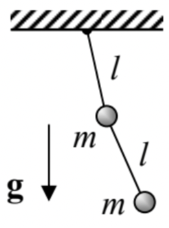
2.1. A double pendulum - see the figure on the right. Consider only the motion in the vertical plane containing the suspension point.

Screen Shot 2022-01-25 at 9.38.29 PM.png

2.2. A stretchable pendulum (i.e. a massive particle hung on an elastic cord that exerts force \(F=-\kappa\left(l-l_{0}\right)\), where \(\kappa\) and \(l_{0}\) are positive constants), also confined to the vertical plane:

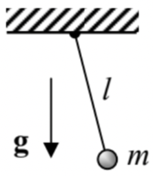
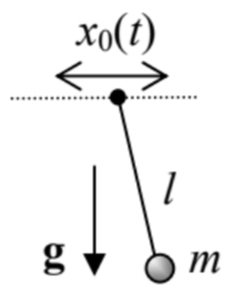
Screen Shot 2022-01-25 at 9.38.56 PM.png

2.3. A fixed-length pendulum hanging from a horizontal support whose motion law \(\ x_{0}(t)\) is fixed. (No vertical plane constraint here.)

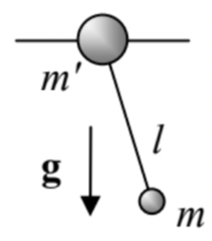
Screen Shot 2022-01-25 at 9.40.19 PM.png

2.4. A pendulum of mass \(m\), hung on another point mass \(m\) ’, which may slide, without friction, along a straight horizontal rail - see the figure on the right. The motion is confined to the vertical plane that contains the rail.

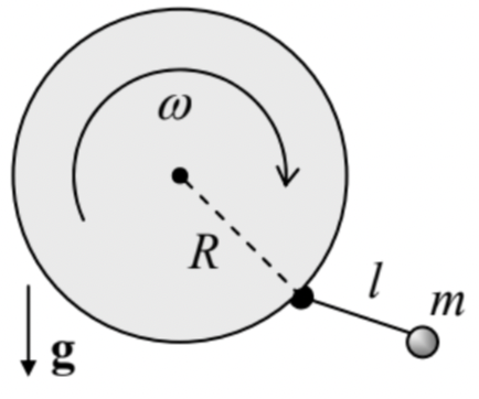
Screen Shot 2022-01-25 at 9.41.12 PM.png

2.5. A point-mass pendulum of length \(l\), attached to the rim of a disk of radius \(R\), which is rotated in a vertical plane with a constant angular velocity \(\omega\) - see the figure on the right. (Consider only the motion within the disk’s plane.)

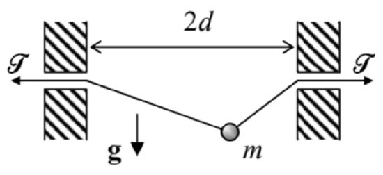
Screen Shot 2022-01-25 at 9.42.00 PM.png

2.6. A bead of mass \(m\), sliding without friction along a light string stretched by a fixed force \(\mathscr{T}\) between two horizontally displaced points \(-\) see the figure on the right. Here, in contrast to the similar Problem 1.10, the string tension \(\mathscr{T}\) may be comparable with the bead’s weight \(m g\), and the motion is not restricted to the vertical plane.

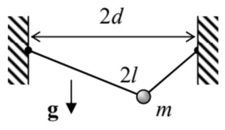
Screen Shot 2022-01-25 at 9.42.27 PM.png

2.7. A bead of mass \(m\), sliding without friction along a light string of a fixed length \(2 l\), which is hung between two points, horizontally displaced by distance \(2 d<2 l-\) see the figure on the right. As in the previous problem, the motion is not restricted to the vertical plane.

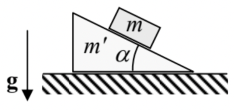
Screen Shot 2022-01-25 at 9.43.09 PM.png

2.8. A block of mass \(m\) that can slide, without friction, along the inclined plane surface of a heavy wedge with mass \(m\) ’. The wedge is free to move, also without friction, along a horizontal surface - see the figure on the right. (Both motions are within the vertical plane containing the steepest slope line.)

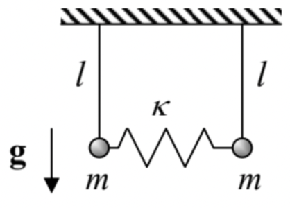
Screen Shot 2022-01-25 at 9.43.47 PM.png

2.9. The two-pendula system that was the subject of Problem 1.8 – see the figure on the right.

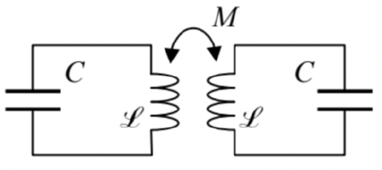
Screen Shot 2022-01-25 at 9.44.51 PM.png

2.10. A system of two similar, inductively-coupled \(\ LC\) circuits – see the figure on the right.

Screen Shot 2022-01-25 at 9.45.43 PM.png

2.11.* A small Josephson junction - the system consisting of two superconductors (S) weakly coupled by Cooper-pair tunneling through a thin insulating layer (I) that separates them - see the figure on the right.

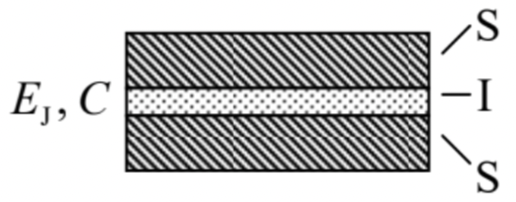
Screen Shot 2022-01-25 at 9.46.37 PM.png

Hints:

(i) At not very high frequencies (whose quantum \(\hbar \omega\) is lower than the binding energy \(2 \Delta\) of the Cooper pairs), the Josephson effect in a sufficiently small junction may be described by the following coupling energy: \[U(\varphi)=-E_{\mathrm{J}} \cos \varphi+\text { const }\] where the constant \(E_{J}\) describes the coupling strength, while the variable \(\varphi\) (called the Josephson phase difference) is connected to the voltage \(V\) across the junction by the famous frequency-to-voltage relation \[\frac{d \varphi}{d t}=\frac{2 e}{\hbar} V,\] where \(e \approx 1.602 \times 10^{-19} \mathrm{C}\) is the fundamental electric charge and \(\hbar \approx 1.054 \times 10^{-34} \mathrm{~J} \cdot \mathrm{s}\) is the Planck constant. \({ }^{18}\)

(ii) The junction (as any system of two close conductors) has a substantial electric capacitance \(C\).

\({ }^{18}\) More discussion of the Josephson effect and the physical sense of the variable \(\varphi\) may be found, for example, in EM Sec. \(6.5\) and QM Secs. \(1.6\) and \(2.8\) of this lecture note series, but the given problem may be solved without that additional information.