
2.2: Three Simple Examples
- Page ID
- 34746

\( \newcommand{\vecs}[1]{\overset { \scriptstyle \rightharpoonup} {\mathbf{#1}} } \)
\( \newcommand{\vecd}[1]{\overset{-\!-\!\rightharpoonup}{\vphantom{a}\smash {#1}}} \)
\( \newcommand{\dsum}{\displaystyle\sum\limits} \)
\( \newcommand{\dint}{\displaystyle\int\limits} \)
\( \newcommand{\dlim}{\displaystyle\lim\limits} \)
\( \newcommand{\id}{\mathrm{id}}\) \( \newcommand{\Span}{\mathrm{span}}\)
( \newcommand{\kernel}{\mathrm{null}\,}\) \( \newcommand{\range}{\mathrm{range}\,}\)
\( \newcommand{\RealPart}{\mathrm{Re}}\) \( \newcommand{\ImaginaryPart}{\mathrm{Im}}\)
\( \newcommand{\Argument}{\mathrm{Arg}}\) \( \newcommand{\norm}[1]{\| #1 \|}\)
\( \newcommand{\inner}[2]{\langle #1, #2 \rangle}\)
\( \newcommand{\Span}{\mathrm{span}}\)
\( \newcommand{\id}{\mathrm{id}}\)
\( \newcommand{\Span}{\mathrm{span}}\)
\( \newcommand{\kernel}{\mathrm{null}\,}\)
\( \newcommand{\range}{\mathrm{range}\,}\)
\( \newcommand{\RealPart}{\mathrm{Re}}\)
\( \newcommand{\ImaginaryPart}{\mathrm{Im}}\)
\( \newcommand{\Argument}{\mathrm{Arg}}\)
\( \newcommand{\norm}[1]{\| #1 \|}\)
\( \newcommand{\inner}[2]{\langle #1, #2 \rangle}\)
\( \newcommand{\Span}{\mathrm{span}}\) \( \newcommand{\AA}{\unicode[.8,0]{x212B}}\)
\( \newcommand{\vectorA}[1]{\vec{#1}} % arrow\)
\( \newcommand{\vectorAt}[1]{\vec{\text{#1}}} % arrow\)
\( \newcommand{\vectorB}[1]{\overset { \scriptstyle \rightharpoonup} {\mathbf{#1}} } \)
\( \newcommand{\vectorC}[1]{\textbf{#1}} \)
\( \newcommand{\vectorD}[1]{\overrightarrow{#1}} \)
\( \newcommand{\vectorDt}[1]{\overrightarrow{\text{#1}}} \)
\( \newcommand{\vectE}[1]{\overset{-\!-\!\rightharpoonup}{\vphantom{a}\smash{\mathbf {#1}}}} \)
\( \newcommand{\vecs}[1]{\overset { \scriptstyle \rightharpoonup} {\mathbf{#1}} } \)
\(\newcommand{\longvect}{\overrightarrow}\)
\( \newcommand{\vecd}[1]{\overset{-\!-\!\rightharpoonup}{\vphantom{a}\smash {#1}}} \)
\(\newcommand{\avec}{\mathbf a}\) \(\newcommand{\bvec}{\mathbf b}\) \(\newcommand{\cvec}{\mathbf c}\) \(\newcommand{\dvec}{\mathbf d}\) \(\newcommand{\dtil}{\widetilde{\mathbf d}}\) \(\newcommand{\evec}{\mathbf e}\) \(\newcommand{\fvec}{\mathbf f}\) \(\newcommand{\nvec}{\mathbf n}\) \(\newcommand{\pvec}{\mathbf p}\) \(\newcommand{\qvec}{\mathbf q}\) \(\newcommand{\svec}{\mathbf s}\) \(\newcommand{\tvec}{\mathbf t}\) \(\newcommand{\uvec}{\mathbf u}\) \(\newcommand{\vvec}{\mathbf v}\) \(\newcommand{\wvec}{\mathbf w}\) \(\newcommand{\xvec}{\mathbf x}\) \(\newcommand{\yvec}{\mathbf y}\) \(\newcommand{\zvec}{\mathbf z}\) \(\newcommand{\rvec}{\mathbf r}\) \(\newcommand{\mvec}{\mathbf m}\) \(\newcommand{\zerovec}{\mathbf 0}\) \(\newcommand{\onevec}{\mathbf 1}\) \(\newcommand{\real}{\mathbb R}\) \(\newcommand{\twovec}[2]{\left[\begin{array}{r}#1 \\ #2 \end{array}\right]}\) \(\newcommand{\ctwovec}[2]{\left[\begin{array}{c}#1 \\ #2 \end{array}\right]}\) \(\newcommand{\threevec}[3]{\left[\begin{array}{r}#1 \\ #2 \\ #3 \end{array}\right]}\) \(\newcommand{\cthreevec}[3]{\left[\begin{array}{c}#1 \\ #2 \\ #3 \end{array}\right]}\) \(\newcommand{\fourvec}[4]{\left[\begin{array}{r}#1 \\ #2 \\ #3 \\ #4 \end{array}\right]}\) \(\newcommand{\cfourvec}[4]{\left[\begin{array}{c}#1 \\ #2 \\ #3 \\ #4 \end{array}\right]}\) \(\newcommand{\fivevec}[5]{\left[\begin{array}{r}#1 \\ #2 \\ #3 \\ #4 \\ #5 \\ \end{array}\right]}\) \(\newcommand{\cfivevec}[5]{\left[\begin{array}{c}#1 \\ #2 \\ #3 \\ #4 \\ #5 \\ \end{array}\right]}\) \(\newcommand{\mattwo}[4]{\left[\begin{array}{rr}#1 \amp #2 \\ #3 \amp #4 \\ \end{array}\right]}\) \(\newcommand{\laspan}[1]{\text{Span}\{#1\}}\) \(\newcommand{\bcal}{\cal B}\) \(\newcommand{\ccal}{\cal C}\) \(\newcommand{\scal}{\cal S}\) \(\newcommand{\wcal}{\cal W}\) \(\newcommand{\ecal}{\cal E}\) \(\newcommand{\coords}[2]{\left\{#1\right\}_{#2}}\) \(\newcommand{\gray}[1]{\color{gray}{#1}}\) \(\newcommand{\lgray}[1]{\color{lightgray}{#1}}\) \(\newcommand{\rank}{\operatorname{rank}}\) \(\newcommand{\row}{\text{Row}}\) \(\newcommand{\col}{\text{Col}}\) \(\renewcommand{\row}{\text{Row}}\) \(\newcommand{\nul}{\text{Nul}}\) \(\newcommand{\var}{\text{Var}}\) \(\newcommand{\corr}{\text{corr}}\) \(\newcommand{\len}[1]{\left|#1\right|}\) \(\newcommand{\bbar}{\overline{\bvec}}\) \(\newcommand{\bhat}{\widehat{\bvec}}\) \(\newcommand{\bperp}{\bvec^\perp}\) \(\newcommand{\xhat}{\widehat{\xvec}}\) \(\newcommand{\vhat}{\widehat{\vvec}}\) \(\newcommand{\uhat}{\widehat{\uvec}}\) \(\newcommand{\what}{\widehat{\wvec}}\) \(\newcommand{\Sighat}{\widehat{\Sigma}}\) \(\newcommand{\lt}{<}\) \(\newcommand{\gt}{>}\) \(\newcommand{\amp}{&}\) \(\definecolor{fillinmathshade}{gray}{0.9}\)As the first, simplest example, consider a particle constrained to move along one axis (say, \(x\) ): \[T=\frac{m}{2} \dot{x}^{2}, \quad U=U(x, t) .\] In this case, it is natural to consider \(x\) as the (only) generalized coordinate, and \(\dot{x}\) as the generalized velocity, so that \[L \equiv T-U=\frac{m}{2} \dot{x}^{2}-U(x, t) .\] Considering \(\dot{x}\) as an independent variable, we get \(\partial L / \partial \dot{x}=m \dot{x}\), and \(\partial L / \partial x=-\partial U / \partial x\), so that Eq. (19) (the only Lagrange equation in this case of the single degree of freedom!) yields
\[\frac{d}{d t}(m \dot{x})-\left(-\frac{\partial U}{\partial x}\right)=0\] evidently the same result as the \(x\)-component of the \(2^{\text {nd }}\) Newton law with \(F_{x}=-\partial U / \partial x\). This example is a good sanity check, but it also shows that the Lagrange formalism does not provide too much advantage in this particular case.
Such an advantage is, however, evident for our testbed problem - see Figure 1. Indeed, taking the polar angle \(\theta\) for the (only) generalized coordinate, we see that in this case, the kinetic energy depends not only on the generalized velocity but also on the generalized coordinate: 9 \[\begin{aligned} &T=\frac{m}{2} R^{2}\left(\dot{\theta}^{2}+\omega^{2} \sin ^{2} \theta\right), \quad U=-m g z+\text { const } \equiv-m g R \cos \theta+\text { const }, \\ &L \equiv T-U=\frac{m}{2} R^{2}\left(\dot{\theta}^{2}+\omega^{2} \sin ^{2} \theta\right)+m g R \cos \theta+\text { const. } \end{aligned}\] Here it is especially important to remember that at substantiating the Lagrange equation, \(\theta\) and \(\dot{\theta}\) have to be treated as independent arguments of \(L\), so that \[\frac{\partial L}{\partial \dot{\theta}}=m R^{2} \dot{\theta}, \quad \frac{\partial L}{\partial \theta}=m R^{2} \omega^{2} \sin \theta \cos \theta-m g R \sin \theta,\] giving us the following equation of motion: \[\frac{d}{d t}\left(m R^{2} \dot{\theta}\right)-\left(m R^{2} \omega^{2} \sin \theta \cos \theta-m g R \sin \theta\right)=0 .\] As a sanity check, at \(\omega=0\), Eq. (25) is reduced to the equation (1.18) of the usual pendulum: \[\ddot{\theta}+\Omega^{2} \sin \theta=0, \quad \text { where } \Omega \equiv\left(\frac{g}{R}\right)^{1 / 2} .\] We will explore the full dynamic equation (25) in more detail later, but please note how simple its derivation was - in comparison with writing the 3D Newton law and then excluding the reaction force.
Next, though the Lagrangian formalism was derived from the Newton law for mechanical systems, the resulting equations (19) are applicable to other dynamic systems, especially those for which the kinetic and potential energies may be readily expressed via some generalized coordinates. As the simplest example, consider the well-known connection (Figure 4) of a capacitor with capacitance \(C\) to an inductive coil with self-inductance \(\mathscr{L}^{0}\) (Electrical engineers frequently call it the \(L C\) tank circuit.)
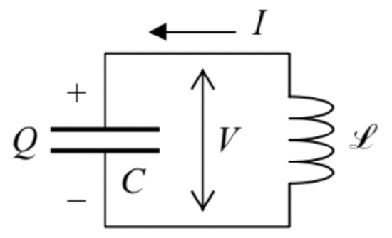
As the reader (hopefully :-) knows, at relatively low frequencies we may use the so-called lumped-circuit approximation, in which the total energy of the system is the sum of two components, the electric energy \(E_{\mathrm{e}}\) localized inside the capacitor, and the magnetic energy \(E_{\mathrm{m}}\) localized inside the inductance coil: \[E_{\mathrm{e}}=\frac{Q^{2}}{2 C}, \quad E_{\mathrm{m}}=\frac{\mathscr{L} I^{2}}{2} .\] Since the electric current \(I\) through the coil and the electric charge \(Q\) on the capacitor are connected by the charge continuity equation \(d Q / d t=I\) (evident from Figure 4), it is natural to declare the charge the generalized coordinate of the system, and the current, its generalized velocity. With this choice, the electrostatic energy \(E_{\mathrm{e}}(Q)\) may be treated as the potential energy \(U\) of the system, and the magnetic energy \(E_{\mathrm{m}}(I)\), as its kinetic energy \(T\). With this attribution, we get \[\frac{\partial T}{\partial \dot{q}} \equiv \frac{\partial E_{\mathrm{m}}}{\partial I}=\mathscr{L} I \equiv \mathscr{L} \dot{Q}, \quad \frac{\partial T}{\partial q} \equiv \frac{\partial E_{\mathrm{m}}}{\partial Q}=0, \quad \frac{\partial U}{\partial q} \equiv \frac{\partial E_{\mathrm{e}}}{\partial Q}=\frac{Q}{C},\] so that the Lagrange equation (19) becomes \[\frac{d}{d t}(\mathscr{L} \dot{Q})-\left(-\frac{Q}{C}\right)=0 .\] Note, however, that the above choice of the generalized coordinate and velocity is not unique. Instead, one can use, as the generalized coordinate, the magnetic flux \(\Phi\) through the inductive coil, related to the common voltage \(V\) across the circuit (Figure 4) by Faraday’s induction law \(V=-d \Phi / d t\). With this choice, \((-V)\) becomes the generalized velocity, \(E_{\mathrm{m}}=\Phi^{2} / 2 \mathscr{L}\) should be understood as the potential energy, and \(E_{\mathrm{e}}=C V^{2} / 2\) treated as the kinetic energy. For this choice, the resulting Lagrange equation of motion is equivalent to Eq. (29). If both parameters of the circuit, \(\mathscr{L}\) and \(C\), are constant in time, Eq. (29) is just the harmonic oscillator equation and describes sinusoidal oscillations with the frequency \[\omega_{0}=\frac{1}{(\mathscr{C} C)^{1 / 2}} .\] This is of course a well-known result, which may be derived in a more standard way - by equating the voltage drops across the capacitor \((V=Q / C)\) and the inductor \(\left(V=-\mathscr{L} d I / d t \equiv-\mathscr{l} d^{2} Q / d t^{2}\right)\). However, the Lagrangian approach is much more convenient for more complex systems - for example, for the general description of the electromagnetic field and its interaction with charged particles. \({ }^{11}\)
\({ }^{9}\) The above expression for \(T \equiv(m / 2)\left(\dot{x}^{2}+\dot{y}^{2}+\dot{z}^{2}\right)\) may be readily obtained either by the formal differentiation of Eq. (2) over time, or just by noticing that the velocity vector has two perpendicular components: one (of magnitude \(R \dot{\theta}\) ) along the ring, and another one (of magnitude \(\omega \rho=\omega R \sin \theta\) ) normal to the ring’s plane.
\({ }^{10}\) A fancy font is used here to avoid any chance of confusion between the inductance and the Lagrange function.
\({ }^{11}\) See, e.g., EM Secs. \(9.7\) and 9.8.