3.2: Equilibrium and Stability

Autonomous systems are defined as dynamic systems whose equations of motion do not depend on time explicitly. For the effectively-1D (and in particular the really-1D) systems obeying Eq. (4), this means that their function \(U_{\mathrm{ef}}\), and hence the Lagrangian function (3) should not depend on time explicitly. According to Eqs. (2.35), in such systems, the Hamiltonian function (7), i.e. the sum \(T_{\text {ef }}+U_{\text {ef, }}\) is an integral of motion. However, be careful! Generally, this conclusion is not valid for the mechanical energy \(E\) of such a system; for example, as we already know from Sec. 2.2, for our testbed problem, with the generalized coordinate \(q=\theta\) (Figure 2.1), \(E\) is not conserved.

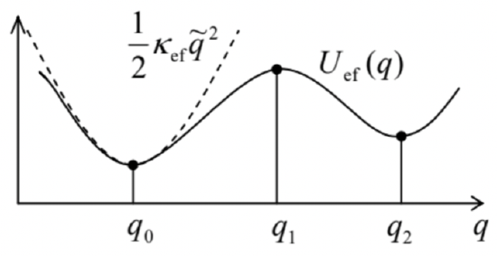
According to Eq. (4), an autonomous system, at appropriate initial conditions, may stay in equilibrium at one or several stationary (alternatively called fixed) points \(q_{n}\), corresponding to either the minimum or a maximum of the effective potential energy (see Figure 1): \[\frac{d U_{\mathrm{ef}}}{d q}\left(q_{n}\right)=0\]

Figure 3.1. The effective potential energy profile near stable \(\ \left(q_{0}, q_{2}\right)\) and unstable \(\ \left(q_{1}\right)\) fixed points, and its quadratic approximation (10) near point \(\ q_{0}\) - schematically.

In order to explore the stability of such fixed points, let us analyze the dynamics of small deviations \[\widetilde{q}(t) \equiv q(t)-q_{n}\] from the equilibrium. For that, let us expand the function \(U_{\text {ef }}(\mathrm{q})\) in the Taylor series at a fixed point: \[U_{\mathrm{ef}}(q)=U_{\mathrm{ef}}\left(q_{n}\right)+\frac{d U_{\mathrm{ef}}}{d q}\left(q_{n}\right) \widetilde{q}+\frac{1}{2} \frac{d^{2} U_{\mathrm{ef}}}{d q^{2}}\left(q_{n}\right) \widetilde{q}^{2}+\ldots\] The first term on the right-hand side, \(U_{\text {ef }}\left(q_{n}\right)\), is arbitrary and does not affect motion. The next term, linear in deviation \(\widetilde{q}\), equals zero - see the fixed point’s definition (8). Hence the fixed point stability is determined by the next term, quadratic in \(\widetilde{q}\), more exactly by its coefficient, \[\kappa_{\mathrm{ef}} \equiv \frac{d^{2} U_{\mathrm{ef}}}{d q^{2}}\left(q_{n}\right),\] which plays the role of the effective spring constant. Indeed, neglecting the higher terms of the Taylor expansion \((10),{ }^{1}\) we see that Eq. (4) takes the familiar form: \[m_{\mathrm{ef}} \ddot{\widetilde{q}}+\kappa_{\mathrm{ef}} \widetilde{q}=0 .\] I am confident that the reader of these notes knows everything about this equation, but since we will soon run into similar but more complex equations, let us review the formal procedure of its solution. From the mathematical standpoint, Eq. (12) is an ordinary, linear differential equation of the second order, with constant coefficients. The theory of such equations tells us that its general solution (for any initial conditions) may be represented as \[\widetilde{q}(t)=c_{+} e^{\lambda_{+} t}+c_{-} e^{\lambda_{-} t},\] where the constants \(c_{\pm}\)are determined by initial conditions, while the so-called characteristic exponents \(\lambda_{\pm}\)are completely defined by the equation itself. To calculate these exponents, it is sufficient to plug just one partial solution, \(e^{\lambda t}\), into the equation. In our simple case (12), this yields the following characteristic equation: \[m_{\mathrm{ef}} \lambda^{2}+\kappa_{\mathrm{ef}}=0 .\] If the ratio \(k_{\mathrm{ef}} / m_{\mathrm{ef}}\) is positive, i.e. the fixed point corresponds to the minimum of potential energy (e.g., see points \(q_{0}\) or \(q_{2}\) in Figure 1), the characteristic equation yields \[\lambda_{\pm}=\pm i \omega_{0}, \quad \text { with } \omega_{0} \equiv\left(\frac{\kappa_{\text {ef }}}{m_{\text {ef }}}\right)^{1 / 2},\] (where \(i\) is the imaginary unit, \(i^{2}=-1\) ), so that Eq. (13) describes sinusoidal oscillations of the system, \({ }^{2}\) \[\widetilde{q}(t)=c_{+} e^{+i \omega_{0} t}+c_{-} e^{-i \omega_{0} t} \equiv c_{c} \cos \omega_{0} t+c_{s} \sin \omega_{0} t,\] with the frequency \(\omega_{0}\), about the fixed point - which is thereby stable. \({ }^{3}\) On the other hand, at the potential energy maximum \(\left(k_{\text {ef }}<0\right.\), e.g., at point \(q_{1}\) in Figure 1), we get \[\lambda_{\pm}=\pm \lambda, \quad \lambda \equiv\left(\frac{\left|\kappa_{\mathrm{ef}}\right|}{m_{\mathrm{ef}}}\right)^{1 / 2}, \quad \tilde{q}(t)=c_{+} e^{+\lambda t}+c_{-} e^{-\lambda t}\] Since the solution has an exponentially growing part, \({ }^{4}\) the fixed point is unstable.

Note that the quadratic expansion of function \(U_{\mathrm{ef}}(q)\), given by the truncation of Eq. (10) to the three displayed terms, is equivalent to a linear Taylor expansion of the effective force: \[F_{\text {ef }} \equiv-\frac{d U_{\text {ef }}}{d q} \approx-\kappa_{\text {ef }} \widetilde{q},\] immediately resulting in the linear equation (12). Hence, to analyze the stability of a fixed point \(q_{n}\), it is sufficient to linearize the equation of motion with respect to small deviations from the point, and study possible solutions of the resulting linear equation. This linearization procedure is typically simpler to carry out than the quadratic expansion (10).

As an example, let us return to our testbed problem (Figure 2.1) whose function \(U_{\text {ef }}\) we already know - see the second of Eqs. (6). With it, the equation of motion (4) becomes \[m R^{2} \ddot{\theta}=-\frac{d U_{\mathrm{ef}}}{d \theta}=m R^{2}\left(\omega^{2} \cos \theta-\Omega^{2}\right) \sin \theta, \quad \text { i.e. } \ddot{\theta}=\left(\omega^{2} \cos \theta-\Omega^{2}\right) \sin \theta,\] where \(\Omega \equiv(g / R)^{1 / 2}\) is the frequency of small oscillations of the system at \(\omega=0\) - see Eq. ( \(\left.2.26\right) .^{5}\) From requirement (8), we see that on any \(2 \pi\)-long segment of the angle \(\theta,{ }^{6}\) the system may have four fixed points; for example, on the half-open segment \((-\pi,+\pi]\) these points are \[\theta_{0}=0, \quad \theta_{1}=\pi, \quad \theta_{2,3}=\pm \cos ^{-1} \frac{\Omega^{2}}{\omega^{2}} .\] The last two fixed points, corresponding to the bead shifted to either side of the rotating ring, exist only if the angular velocity \(\omega\) of the rotation exceeds \(\Omega\). (In the limit of very fast rotation, \(\omega>>\Omega\), Eq. (20) yields \(\theta_{2,3} \rightarrow \pm \pi / 2\), i.e. the stationary positions approach the horizontal diameter of the ring - in accordance with our physical intuition.)To analyze the fixed point stability, we may again use Eq. (9), in the form \(\theta=\theta_{n}+\widetilde{\theta}\), plug it into Eq. (19), and Taylor-expand the trigonometric functions of \(\theta\) up to the first term in \(\widetilde{\theta}\) : \[\ddot{\tilde{\theta}}=\left[\omega^{2}\left(\cos \theta_{n}-\sin \theta_{n} \widetilde{\theta}\right)-\Omega^{2}\right]\left(\sin \theta_{n}+\cos \theta_{n} \widetilde{\theta}\right) .\] Generally, this equation may be linearized further by purging its right-hand side of the term proportional to \(\widetilde{\theta}^{2}\); however in this simple case, Eq. (21) is already convenient for analysis. In particular, for the fixed point \(\theta_{0}=0\) (corresponding to the bead’s position at the bottom of the ring), we have \(\cos \theta_{0}=1\) and \(\sin \theta_{0}=0\), so that Eq. (21) is reduced to a linear differential equation \[\ddot{\tilde{\theta}}=\left(\omega^{2}-\Omega^{2}\right) \tilde{\theta} \text {, }\] whose characteristic equation is similar to Eq. (14) and yields \[\lambda^{2}=\omega^{2}-\Omega^{2}, \text { for } \theta \approx \theta_{0} .\] This result shows that if \(\omega<\Omega\), when both roots \(\lambda\) are imaginary, this fixed point is orbitally stable. However, if the rotation speed is increased so that \(\omega>\Omega\), the roots become real, \(\lambda_{\pm}=\left(\omega^{2}-\Omega^{2}\right)^{1 / 2}\), with one of them positive, so that the fixed point becomes unstable beyond this threshold, i.e. as soon as fixed points \(\theta_{2,3}\) exist. Absolutely similar calculations for other fixed points yield \[\lambda^{2}= \begin{cases}\Omega^{2}+\omega^{2}>0, & \text { for } \theta \approx \theta_{1}, \\ \Omega^{2}-\omega^{2}, & \text { for } \theta \approx \theta_{2,3} .\end{cases}\] These results show that the fixed point \(\theta_{1}\) (bead on the top of the ring) is always unstable - just as we could foresee, while the side fixed points \(\theta_{2,3}\) are orbitally stable as soon as they exist (at \(\omega>\Omega\) ).

Thus, our fixed-point analysis may be summarized very simply: an increase of the ring rotation speed \(\omega\) beyond a certain threshold value, equal to \(\Omega\) given by Eq. (2.26), causes the bead to move to one of the ring sides, oscillating about one of the fixed points \(\theta_{2,3}\). Together with the rotation about the vertical axis, this motion yields quite a complex (generally, open) spatial trajectory as observed from a lab frame, so it is fascinating that we could analyze it quantitatively in such a simple way.

Later in this course, we will repeatedly use the linearization of the equations of motion for the analysis of stability of more complex systems, including those with energy dissipation.

---

\({ }^{1}\) Those terms may be important only in very special cases then \(\kappa_{\text {ef }}\) is exactly zero, i.e. when a fixed point is an inflection point of the function \(U_{\mathrm{er}}(q)\).

\({ }^{2}\) The reader should not be scared of the first form of (16), i.e. of the representation of a real variable (the deviation from equilibrium) via a sum of two complex functions. Indeed, any real initial conditions give \(c_{-}^{*}=c_{+}\), so that the sum is real for any \(t\). An even simpler way to deal with such complex representations of real functions will be discussed in the beginning of the next chapter, and then used throughout the series.

\({ }^{3}\) This particular type of stability, when the deviation from the equilibrium oscillates with a constant amplitude, neither growing nor decreasing in time, is called either the orbital, or "neutral", or "indifferent" stability.

\({ }^{4}\) Mathematically, the growing part vanishes at some special (exact) initial conditions which give \(c_{+}=0\). However, the futility of this argument for real physical systems should be obvious for anybody who had ever tried to balance a pencil on its sharp point.

\({ }^{5}\) Note that Eq. (19) coincides with Eq. (2.25). This is a good sanity check illustrating that the procedure (5)-(6) of moving of a term from the potential to the kinetic energy within the Lagrangian function is indeed legitimate.

\({ }^{6}\) For this particular problem, the values of \(\theta\) that differ by a multiple of \(2 \pi\), are physically equivalent.