
3.3: Hamiltonian 1D Systems


- Last updated
- Jan 26, 2022
- Save as PDF

( \newcommand{\kernel}{\mathrm{null}\,}\)
Autonomous systems that are described by time-independent Lagrangians are frequently called Hamiltonian ones because their Hamiltonian function H (again, not necessarily equal to the genuine mechanical energy E! ) is conserved. In our current 1D case, described by Eq. (3), H=mef2˙q2+Uef(q)= const . From the mathematical standpoint, this conservation law is just the first integral of motion. Solving Eq. (24) for ˙q, we get the first-order differential equation, dqdt=±{2mef[H−Uef(q)]}1/2, i.e. ±(mef2)1/2dq[H−Uef(q)]1/2=dt, which may be readily integrated: ±(mef2)1/2∫q(t)q(t0)dq′[H−Uef(q′)]1/2=t−t0. Since the constant H (as well as the proper sign before the integral - see below) is fixed by initial conditions, Eq. (26) gives the reciprocal form, t=t(q), of the desired law of system motion, q(t). Of course, for any particular problem the integral in Eq. (26) still has to be worked out, either analytically or numerically, but even the latter procedure is typically much easier than the numerical integration of the initial, second-order differential equation of motion, because at the addition of many values (to which any numerical integration is reduced 7 ) the rounding errors are effectively averaged out.
Moreover, Eq. (25) also allows a general classification of 1D system motion. Indeed:
(i) If H>Uef(q) in the whole range of interest, the effective kinetic energy Tef (3) is always positive. Hence the derivative dq/dt cannot change its sign, so that the effective velocity retains the sign it had initially. This is an unbound motion in one direction (Figure 2a).
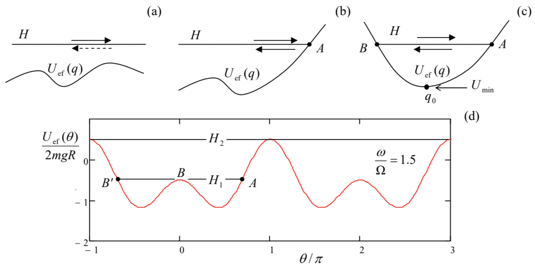
(ii) Now let the particle approach a classical turning point A where H=Uef(q)−seeFig.2 b.8 According to Eq. (25), at that point the particle velocity vanishes, while its acceleration, according to Eq. (4), is still finite. This corresponds to the particle reflection from this potential wall, with the change of the velocity sign.
(iii) If, after the reflection from point A, the particle runs into another classical turning point B (Figure 2c), the reflection process is repeated again and again, so that the particle is bound to a periodic motion between two turning points.
The last case of periodic oscillations presents a large conceptual and practical interest, and the whole next chapter will be devoted to a detailed analysis of this phenomenon and numerous associated effects. Here I will only note that for an autonomous Hamiltonian system described by Eq. (4), Eq. (26) immediately enables the calculation of the oscillation period: τ=2(mef2)1/2∫ABdq[H−Uef(q)]1/2 where the additional front factor 2 accounts for two time intervals: of the motion from B to A and back see Figure 2c. Indeed, according to Eq. (25), in each classically allowed point q, the velocity magnitude is the same so that these time intervals are equal to each other.
(Note that the dependence of points A and B on H is not necessarily continuous. For example, for our testbed problem, whose effective potential energy is plotted in Figure 2 d for a particular value of ω> Ω, a gradual increase of H leads to a sudden jump, at H=H1, of the point B to a new position B ’, corresponding to a sudden switch from oscillations about one fixed point θ2,3 to oscillations about two adjacent fixed points - before the beginning of a persistent rotation around the ring at H>H2.)
Now let us consider a particular, but very important limit of Eq. (27). As Figure 2c shows, if H is reduced to approach Umin, the periodic oscillations take place at the very bottom of "potential well", about a stable fixed point q0. Hence, if the potential energy profile is smooth enough, we may limit the Taylor expansion (10) to the displayed quadratic term. Plugging it into Eq. (27), and using the mirror symmetry of this particular problem about the fixed point q0, we get τ=4(mef2)1/2∫A0d˜q[H−(Umin+κef˜q2/2)]1/2=4ω0I, with I≡∫10dξ(1−ξ2)1/2 where ξ≡˜q/A, with A≡(2/κef)1/2(H−Umin)1/2 being the classical turning point, i.e. the oscillation amplitude, and ω0 the frequency given by Eq. (15). Taking into account that the elementary integral I in that equation equals π/2,9 we finally get τ=2πω0, as it should be for the harmonic oscillations (16). Note that the oscillation period does not depend on the oscillation amplitude A, i.e. on the difference (H−Umin)− while it is sufficiently small.
7 See, e.g., MA Eqs. (5.2) and (5.3).
8 This terminology comes from quantum mechanics, which shows that a particle (or rather its wavefunction) actually can, to a certain extent, penetrate into the "classically forbidden range" where H<Uef(q).
9 Indeed, introducing a new variable ζ as ξ≡sinζ, we get dξ=cosζdζ=(1−ξ2)1/2dζ, so that the function under the integral is just dζ, and its limits are ζ=0 and ζ=π/2.