6.1: Two Coupled Oscillators

Let us discuss oscillations in systems with several degrees of freedom, starting from the simplest case of two linear (harmonic), dissipation-free, 1D oscillators. If the oscillators are independent of each other, the Lagrangian function of their system may be represented as a sum of two independent terms of the type (5.1): \[L=L_{1}+L_{2}, \quad L_{1,2}=T_{1,2}-U_{1,2}=\frac{m_{1,2}}{2} \dot{q}_{1,2}^{2}-\frac{\kappa_{1,2}}{2} q_{1,2}^{2} .\] Correspondingly, Eqs. (2.19) for \(q_{j}=q_{1,2}\) yields two independent equations of motion of the oscillators, each one being similar to Eq. (5.2): \[m_{1,2} \ddot{q}_{1,2}+m_{1,2} \Omega_{1,2}^{2} q_{1,2}=0, \quad \text { where } \Omega_{1,2}^{2}=\frac{\kappa_{1,2}}{m_{1,2}} .\] (In the context of what follows, \(\Omega_{1,2}\) are sometimes called the partial frequencies.) This means that in this simplest case, an arbitrary motion of the system is just a sum of independent sinusoidal oscillations at two frequencies equal to the partial frequencies (2).

However, as soon as the oscillators are coupled (i.e. interact), the full Lagrangian \(L\) contains an additional mixed term \(L_{\text {int }}\) depending on both generalized coordinates \(q_{1}\) and \(q_{2}\) and/or generalized velocities. As a simple example, consider the system shown in Figure 1, there two small masses \(m_{1,2}\) are constrained to move in only one direction (shown horizontal), and are kept between two stiff walls with three springs.

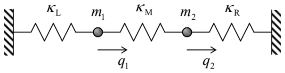Fig. 6.1. A simple system of two coupled linear oscillators.

In this case, the kinetic energy is still separable, \(T=T_{1}+T_{2}\), but the total potential energy, consisting of the elastic energies of three springs, is not: \[U=\frac{\kappa_{\mathrm{L}}}{2} q_{1}^{2}+\frac{\kappa_{\mathrm{M}}}{2}\left(q_{1}-q_{2}\right)^{2}+\frac{\kappa_{\mathrm{R}}}{2} q_{2}^{2},\] where \(q_{1.2}\) are the horizontal displacements of the particles from their equilibrium positions. It is convenient to rewrite this expression as \[U=\frac{\kappa_{1}}{2} q_{1}^{2}+\frac{\kappa_{2}}{2} q_{2}^{2}-\kappa q_{1} q_{2}, \quad \text { where } \kappa_{1} \equiv \kappa_{\mathrm{L}}+\kappa_{\mathrm{M}}, \quad \kappa_{2} \equiv \kappa_{\mathrm{R}}+\kappa_{\mathrm{M}}, \quad \kappa \equiv \kappa_{\mathrm{M}},\] showing that the Lagrangian function \(L=T-U\) of this system contains, besides the partial terms (1), a bilinear interaction term: \[L=L_{1}+L_{2}+L_{\text {int }}, \quad L_{\text {int }}=\kappa q_{1} q_{2} .\] The resulting Lagrange equations of motion are \[\begin{aligned} &m_{1} \ddot{q}_{1}+m_{1} \Omega_{1}^{2} q_{1}=\kappa q_{2}, \\ &m_{2} \ddot{q}_{2}+m_{2} \Omega_{2}^{2} q_{2}=\kappa q_{1} . \end{aligned}\] Thus the interaction leads to an effective generalized force \(\kappa q_{2}\) exerted on subsystem 1 by subsystem 2 , and the reciprocal effective force \(\kappa q_{1}\).

Please note two important aspects of this (otherwise rather simple) system of equations. First, in contrast to the actual physical interaction forces (such as \(F_{12}=-F_{21}=\kappa_{\mathrm{M}}\left(q_{2}-q_{1}\right)\) for our system \(^{1}\) ) the effective forces on the right-hand sides of Eqs. (5) do not obey the \(3^{\text {rd }}\) Newton law. Second, the forces are proportional to the same coefficient \(\kappa\), this feature is a result of the general bilinear structure (4) of the interaction energy, rather than of any special symmetry.

From our prior discussions, we already know how to solve Eqs. (5), because it is still a system of linear and homogeneous differential equations, so that its general solution is a sum of particular solutions of the form similar to Eqs. (5.88), \[q_{1}=c_{1} e^{\lambda t}, \quad q_{2}=c_{2} e^{\lambda t},\] with all possible values of \(\lambda\). These values may be found by plugging Eq. (6) into Eqs. (5), and requiring the resulting system of two linear, homogeneous algebraic equations for the distribution coefficients \(c_{1,2}\), \[\begin{aligned} &m_{1} \lambda^{2} c_{1}+m_{1} \Omega_{1}^{2} c_{1}=\kappa c_{2} \\ &m_{2} \lambda^{2} c_{2}+m_{2} \Omega_{2}^{2} c_{2}=\kappa c_{1} \end{aligned}\] to be self-consistent. In our particular case, we get a characteristic equation, \[\left|\begin{array}{cc} m_{1}\left(\lambda^{2}+\Omega_{1}^{2}\right) & -\kappa \\ -\kappa & m_{2}\left(\lambda^{2}+\Omega_{2}^{2}\right) \end{array}\right|=0,\] that is quadratic in \(\lambda^{2}\), and thus allows a simple analytical solution: \[\left(\lambda^{2}\right)_{\pm}=-\frac{1}{2}\left(\Omega_{1}^{2}+\Omega_{2}^{2}\right) \mp\left[\frac{1}{4}\left(\Omega_{1}^{2}+\Omega_{2}^{2}\right)^{2}-\Omega_{1}^{2} \Omega_{2}^{2}+\frac{\kappa^{2}}{m_{1} m_{2}}\right]^{1 / 2}\] \[\equiv-\frac{1}{2}\left(\Omega_{1}^{2}+\Omega_{2}^{2}\right) \mp\left[\frac{1}{4}\left(\Omega_{1}^{2}-\Omega_{2}^{2}\right)^{2}+\frac{\kappa^{2}}{m_{1} m_{2}}\right]^{1 / 2} .\] According to Eqs. (2) and (3b), for any positive values of spring constants, the product \(\Omega_{1} \Omega_{2}=\) \(\left(\kappa_{L}+\kappa_{M}\right)\left(\kappa_{R}+\kappa_{M}\right) /\left(m_{1} m_{2}\right)^{1 / 2}\) is always larger than \(\kappa /\left(m_{1} m_{2}\right)^{1 / 2}=\kappa_{M} /\left(m_{1} m_{2}\right)^{1 / 2}\), so that the square root in Eq. (9) is always smaller than \(\left(\Omega_{1}{ }^{2}+\Omega_{2}{ }^{2}\right) / 2\). As a result, both values of \(\lambda^{2}\) are negative, i.e. the general solution to Eq. (5) is a sum of four terms, each proportional to \(\exp \left\{\pm i \omega_{\pm} t\right\}\), where both own frequencies ("eigenfrequencies") \(\omega_{\pm} \equiv i \lambda_{\pm}\)are real:

\[\ \text{Anticrossing description}\quad\quad\quad\quad\omega_{\pm}^{2} \equiv-\lambda_{\pm}^{2}=\frac{1}{2}\left(\Omega_{1}^{2}+\Omega_{2}^{2}\right) \pm\left[\frac{1}{4}\left(\Omega_{1}^{2}-\Omega_{2}^{2}\right)^{2}+\frac{\kappa^{2}}{m_{1} m_{2}}\right]^{1 / 2}.\]

A plot of these eigenfrequencies as a function of one of the partial frequencies (say, \(\Omega_{1}\) ), with the other partial frequency fixed, gives us the famous anticrossing (also called the "avoided crossing" or "non-crossing") diagram - see Figure 2. One can see that at weak coupling, frequencies \(\omega_{\pm}\)are close to the partial frequencies \(\Omega_{1,2}\) everywhere besides a narrow range near the anticrossing point \(\Omega_{1}=\Omega_{2}\). Most remarkably, at passing through this region, \(\omega_{+}\)smoothly "switches" from following \(\Omega_{2}\) to following \(\Omega_{1}\) and vice versa.

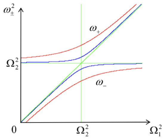
Figure 6.2. The anticrossing diagram for two values of the normalized coupling strength \(\kappa /\left(m_{1} m_{2}\right)^{1 / 2} \Omega_{2}^{2}: 0.3\) (red lines) and \(0.1\) (blue lines). In this plot, \(\Omega_{1}\) is assumed to be changed by varying \(\kappa_{1}\) rather than \(m_{1}\), but in the opposite case, the diagram is qualitatively similar.

The reason for this counterintuitive behavior may be found by examining the distribution coefficients \(c_{1,2}\) corresponding to each branch of the diagram, which may be obtained by plugging the corresponding value of \(\lambda_{\pm}=-i \omega_{\pm}\)back into Eqs. (7). For example, at the anticrossing point \(\Omega_{1}=\Omega_{2} \equiv \Omega\), Eq. (10) is reduced to \[\omega_{\pm}^{2}=\Omega^{2} \pm \frac{\kappa}{\left(m_{1} m_{2}\right)^{1 / 2}}=\Omega^{2}\left(1 \pm \frac{\kappa}{\left(\kappa_{1} \kappa_{2}\right)^{1 / 2}}\right) .\] Plugging this expression back into any of Eqs. (7), we see that for the two branches of the anticrossing diagram, the distribution coefficient ratio is the same by magnitude but opposite by sign: \[\left(\frac{c_{1}}{c_{2}}\right)_{\pm}=\mp\left(\frac{m_{2}}{m_{1}}\right)^{1 / 2}, \text { at } \Omega_{1}=\Omega_{2} .\] In particular, if the system is symmetric \(\left(m_{1}=m_{2}, \kappa_{\mathrm{L}}=\kappa_{\mathrm{R}}\right)\), then at the upper branch, corresponding to \(\omega_{+}>\omega_{-}\), we get \(c_{1}=-c_{2}\). This means that in this so-called hard mode, \({ }^{2}\) masses oscillate in anti-phase: \(q_{1}(t) \equiv-q_{2}(t)\). The resulting substantial extension/compression of the middle spring (see Figure 1 again) yields additional returning force which increases the oscillation frequency. On the contrary, at the lower branch, corresponding to \(\omega_{\text {., the particle oscillations are in phase: } c_{1}}=c_{2}\), i.e. \(q_{1}(t) \equiv q_{2}(t)\), so that the middle spring is neither stretched nor compressed at all. As a result, in this soft mode, the oscillation frequency \(\omega_{-}\)is lower than \(\omega_{+}\), and does not depend on \(\kappa_{\mathrm{M}}\) : \[\omega_{-}^{2}=\Omega^{2}-\frac{\kappa}{m}=\frac{\kappa_{\mathrm{L}}}{m}=\frac{\kappa_{\mathrm{R}}}{m} .\] Note that for both modes, the oscillations equally engage both particles.

Far from the anticrossing point, the situation is completely different. Indeed, a similar calculation of \(c_{1,2}\) shows that on each branch of the diagram, the magnitude of one of the distribution coefficients is much larger than that of its counterpart. Hence, in this limit, any particular mode of oscillations involves virtually only one particle. A slow change of system parameters, bringing it through the anticrossing, results, first, in a maximal delocalization of each mode at \(\Omega_{1}=\Omega_{2}\), and then in the restoration of the localization, but in a different partial degree of freedom.

We could readily carry out similar calculations for the case when the systems are coupled via their velocities, \(L_{\text {int }}=m \dot{q}_{1} \dot{q}_{2}\), where \(m\) is a coupling coefficient \(-\) not necessarily a certain physical mass. \({ }^{3}\) The results are generally similar to those discussed above, again with the maximum level splitting at \(\Omega_{1}=\Omega_{2} \equiv \Omega\) : \[\omega_{\pm}^{2}=\frac{\Omega^{2}}{1 \mp|m| /\left(m_{1} m_{2}\right)^{1 / 2}} \approx \Omega^{2}\left[1 \pm \frac{|m|}{\left(m_{1} m_{2}\right)^{1 / 2}}\right],\] the last relation being valid for weak coupling. The generalization to the case of both coordinate and velocity coupling is also straightforward - see the next section.

Note that the anticrossing diagram, shown in Figure 2, is even more ubiquitous in quantum mechanics, because, due to the time-oscillatory character of the Schrödinger equation solutions, a weak coupling of any two quantum states leads to qualitatively similar behavior of the eigenfrequencies \(\omega_{\pm}\)of the system, and hence of its eigenenergies ("energy levels") \(E_{\pm}=\hbar \omega_{\pm}\)of the system.

One more property of weakly coupled oscillators, a periodic slow transfer of energy from one oscillator to the other and back, especially well pronounced at or near the anticrossing point \(\Omega_{1}=\Omega_{2}\), is also more important for quantum than for classical mechanics. This is why I refer the reader to the QM part of this series for a detailed discussion of this phenomenon.

---

\({ }^{1}\) Using these expressions, Eqs. (5) may be readily obtained from the Newton laws, but the Lagrangian approach used above will make their generalization, in the next section, more straightforward.

\({ }^{2}\) In physics, the term "mode" is typically used to describe the distribution of a variable in space, at its oscillations with a single frequency. In our current case, when the notion of space is reduced to two oscillator numbers, the "mode" means just a set of two distribution coefficients \(c_{1,2}\) for a particular eigenfrequency.

\({ }^{3}\) In mechanics, with \(q_{1,2}\) standing for the actual linear displacements of particles, such coupling is not very natural, but there are many dynamic systems of non-mechanical nature in which such coupling is the most natural one. The simplest example is the system of two \(L C\) ("tank") circuits, with either capacitive or inductive coupling. Indeed, as was discussed in Sec. 2.2, for such a system, the very notions of the potential and kinetic energies are conditional and interchangeable.