7.1: Strain

As was discussed in Chapters 4 and 6, in a continuum, i.e. a system of particles so close to each other that the system discreteness may be neglected, the particle displacement \(\mathbf{q}\) may be considered as a continuous function of space and time. In this chapter, we will consider only small deviations from the rigid-body approximation discussed in Chapter 4, i.e. small deformations. The deformation smallness allows one to consider the displacement vector \(\mathbf{q}\) as a function of the initial (pre-deformation) position of the particle, \(\mathbf{r}\), and time \(t\) - just as was done in Chapter 6 for 1D waves.

The first task of the deformation theory is to exclude from consideration the types of motion considered in Chapter 4, namely the translation and rotation, unrelated to deformations. This means, first of all, that the variables describing deformations should not depend on the part of displacement distribution, that is independent of the position \(\mathbf{r}\) (i.e. is common for the whole media), because that part corresponds to a translational shift rather than to a deformation (Figure 1a). Moreover, even certain nonuniform displacements do not contribute to deformation. For example, Eq. (4.9) (with \(d \mathbf{r}\) replaced with \(d \mathbf{q}\) to comply with our current notation) shows that a small displacement of the type \[d \mathbf{q}_{\text {rotation }}=d \varphi \times \mathbf{r} \text {, }\] where \(d \varphi=\omega d t\) is an infinitesimal vector common for the whole continuum, corresponds to its rotation about the direction of that vector, and has nothing to do with its deformation (Figure 1b).

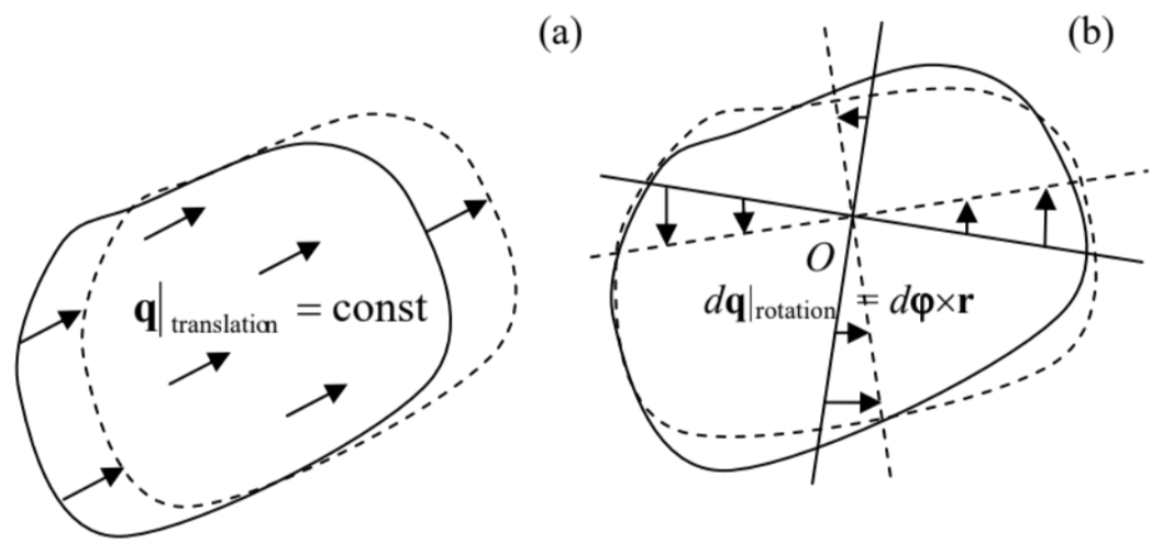Figure 7.1. Two types of displacement vector distributions that are unrelated to deformation: (a) translation and (b) rotation.

This is why to develop an adequate quantitative characterization of deformation, we should start with finding suitable functions of the spatial distribution of displacements, \(\mathbf{q}(\mathbf{r})\), that exist only due to deformations. One of such measures is the change of the distance \(d l=|d \mathbf{r}|\) between two close points: \[\left.(d l)^{2}\right|_{\text {after deformation }}-\left.(d l)^{2}\right|_{\text {before deformation }}=\sum_{j=1}^{3}\left(d r_{j}+d q_{j}\right)^{2}-\sum_{j=1}^{3}\left(d r_{j}\right)^{2}\] where \(d q_{j}\) is the \(j^{\text {th }}\) Cartesian component of the difference \(d \mathbf{q}\) between the displacements \(\mathbf{q}\) of these close points. If the deformation is small in the sense \(|d \mathbf{q}|<<|d \mathbf{r}|=d l\), we may keep in Eq. (2) only the terms proportional to the first power of the infinitesimal vector \(d \mathbf{q}\) : \[\left.(d l)^{2}\right|_{\text {after deformation }}-\left.(d l)^{2}\right|_{\text {before deformation }}=\sum_{j=1}^{3}\left[2 d r_{j} d q_{j}+\left(d q_{j}\right)^{2}\right] \approx 2 \sum_{j=1}^{3} d r_{j} d q_{j} .\] Since \(q_{j}\) is a function of three independent scalar arguments \(r_{j}\), its full differential (at fixed time) may be represented as \[d q_{j}=\sum_{j^{\prime}=1}^{3} \frac{\partial q_{j}}{\partial r_{j^{\prime}}} d r_{j^{\prime}}\] The coefficients \(\partial q_{j} / \partial r_{j}\), may be considered as elements of a tensor \({ }^{1}\) providing a linear relation between the vectors \(\mathrm{d} \mathbf{r}\) and \(\mathrm{d} \mathbf{q}\). Plugging Eq. (4) into Eq. (2), we get \[\left.(d l)^{2}\right|_{\text {after deformation }}-(d l)_{\mid \text {before deformation }}^{2}=2 \sum_{j, j^{\prime}=1}^{3} \frac{\partial q_{j}}{\partial r_{j^{\prime}}} d r_{j} d r_{j^{\prime}} .\] The convenience of the tensor \(\partial q_{j} / \partial r_{j}\), for characterizing deformations is that it automatically excludes the translation displacement (Figure 1a), which is independent of \(r_{j}\). Its drawback is that its particular components are still affected by the rotation of the body (though the sum (5) is not). Indeed, according to the vector product definition, Eq. (1) may be represented in Cartesian coordinates as \[\left.d q_{j}\right|_{\text {rotation }}=\left(d \varphi_{j^{\prime}} r_{j^{\prime \prime}}-d \varphi_{j^{\prime \prime}} r_{j^{\prime}}\right) \varepsilon_{j j j^{\prime \prime}},\] where \(\varepsilon_{i j i j}\) is the Levi-Civita symbol. Differentiating Eq. (6) over a particular Cartesian coordinate of vector \(\mathbf{r}\), and taking into account that this partial differentiation \((\partial)\) is independent of (and hence may be swapped with) the differentiation \((d)\) over the rotation angle \(\varphi\), we get the amounts, \[d\left(\frac{\partial q_{j}}{\partial r_{j^{\prime}}}\right)_{\text {rotation }}=-\varepsilon_{i j j^{\prime \prime}} d \varphi_{j^{\prime \prime}}, \quad d\left(\frac{\partial q_{j^{\prime}}}{\partial r_{j}}\right)_{\text {rotation }}=-\varepsilon_{j i j^{\prime \prime}} d \varphi_{j^{\prime \prime}}=\varepsilon_{j j j^{\prime \prime}} d \varphi_{j^{\prime \prime}},\] which may differ from 0 . However, notice that the sum of these two differentials equals zero for any \(d \varphi\), which is possible only if \(^{2}\) \[\left(\frac{\partial q_{j^{\prime}}}{\partial r_{j}}+\frac{\partial q_{j}}{\partial r_{j^{\prime}}}\right)_{\text {rotation }}=0, \quad \text { for } j \neq j^{\prime} .\] This is why it is convenient to rewrite Eq. (5) in a mathematically equivalent form, \[\left.(d l)^{2}\right|_{\text {affer deformation }}-(d l)^{2} \mid \text { |before deformation }=2 \sum_{j, j^{\prime}=1}^{3} s_{i j^{\prime}} d r_{j} d r_{j^{\prime}} \text {, }\] where \(s_{j j}\) ’ are the elements of the so-called symmetrized strain tensor, defined as \[s_{i j^{\prime}} \equiv \frac{1}{2}\left(\frac{\partial q_{j}}{\partial r_{j^{\prime}}}+\frac{\partial q_{j^{\prime}}}{\partial r_{j}}\right) \text {. }\] (Note that this modification does not affect the diagonal elements: \(s_{j j}=\partial q_{j} / \partial r_{j}\).). The advantage of the symmetrized tensor \((9 \mathrm{~b})\) over the initial tensor with elements \(\partial q_{j} / \partial r_{j}\), is that according to Eq. (8), at pure rotation, all elements of the symmetrized strain tensor vanish.

Now let us discuss the physical meaning of this tensor. As was already mentioned in Sec. 4.2, any symmetric tensor may be diagonalized by an appropriate selection of the reference frame axes. In such principal axes, \(s_{j j}=s_{j j} \delta_{j j}\), so that Eq. (4) takes a simple form: \[d q_{j}=\frac{\partial q_{j}}{\partial r_{j}} d r_{j}=s_{j j} d r_{j} .\] We may use this expression to calculate the change of each side of an elementary cuboid (parallelepiped) with sides \(d q_{j}\) parallel to the principal axes: \[\left.d r_{j}\right|_{\text {after deformation }}-\left.d r_{j}\right|_{\text {before deformation }} \equiv d q_{j}=s_{j j} d r_{j},\] and of cuboid’s volume \(d V=d r_{1} d r_{2} d r_{3}\) : \[\left.d V\right|_{\text {after deformation }}-\left.d V\right|_{\text {before deformation }}=\prod_{j=1}^{3}\left(d r_{j}+s_{j j} d r_{j}\right)-\prod_{j=1}^{3} d r_{j}=d V\left[\prod_{j=1}^{3}\left(1+s_{j j}\right)-1\right]\] Since all our analysis is only valid in the linear approximation in small \(s_{j j}\), Eq. (12) is reduced to \[\left.d V\right|_{\text {after deformation }}-\left.d V\right|_{\text {before deformation }} \approx d V \sum_{j=1}^{3} s_{j j} \equiv d V \operatorname{Tr}(\mathrm{s}),\] where \(\operatorname{Tr}(\text { trace })^{3}\) of any matrix (in particular, any tensor) is the sum of its diagonal elements; in our current case \(^{4}\) \[\operatorname{Tr}(\mathrm{s}) \equiv \sum_{j=1}^{3} s_{j j}\] So, the diagonal components of the tensor characterize the medium’s compression/extension; then what is the meaning of its off-diagonal components? It may be illustrated on the simplest example of purely shear deformation, shown in Figure 2 (the geometry is assumed to be uniform along the \(z\)-axis normal to the plane of the drawing). In this case, all displacements (assumed small) have just one Cartesian component, in Figure 2 along the \(x\)-axis: \(\mathbf{q}=\mathbf{n}_{x} \alpha y\) (with \(\alpha<1\) ), so that the only nonzero component of the initial strain tensor \(\partial q_{j} / \partial r_{j}\), is \(\partial q_{x} / \partial y=\alpha\), and the symmetrized tensor ( \(9 \mathrm{~b}\) ) is \[\mathrm{s}=\left(\begin{array}{ccc} 0 & \alpha / 2 & 0 \\ \alpha / 2 & 0 & 0 \\ 0 & 0 & 0 \end{array}\right) .\] Evidently, the change of volume, given by Eq, (13), vanishes in this case. Thus, off-diagonal elements of the tensor s characterize shear deformations.

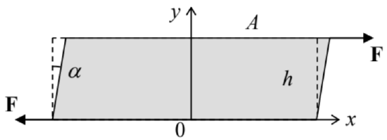Figure 7.2. An example of pure shear.

To conclude this section, let me note that Eq. (9) is only valid in Cartesian coordinates. For the solution of some important problems with the axial or spherical symmetry, it is frequently convenient to express six different components of the symmetric strain tensor via three components of the displacement vector \(\mathbf{q}\) in either cylindrical or spherical coordinates. A straightforward differentiation of the definitions of these curvilinear coordinates, similar to that used to derive the well-known expressions for spatial derivatives, \({ }^{5}\) yields, in particular, the following formulas for the diagonal elements of the tensor:

(i) in the cylindrical coordinates: \[s_{\rho \rho}=\frac{\partial q_{\rho}}{\partial \rho}, \quad s_{\varphi \varphi}=\frac{1}{\rho}\left(q_{r}+\frac{\partial q_{\varphi}}{\partial \varphi}\right), \quad s_{z z}=\frac{\partial q_{z}}{\partial z} .\] (ii) in the spherical coordinates: \[s_{r r}=\frac{\partial q_{r}}{\partial r}, \quad s_{\theta \theta}=\frac{1}{r}\left(q_{r}+\frac{\partial q_{\theta}}{\partial \theta}\right), \quad s_{\varphi \varphi}=\frac{1}{r}\left(q_{r}+q_{\theta} \frac{\cos \theta}{\sin \theta}+\frac{1}{\sin \theta} \frac{\partial q_{\varphi}}{\partial \varphi}\right) .\] These expressions, which will be used below for the solution of some problems for symmetrical geometries, may be a bit counter-intuitive. Indeed, Eq. (16) shows that even for a purely radial, axiallysymmetric deformation, \(\mathbf{q}=\mathbf{n}_{\rho} q(\rho)\), the angular component of the strain tensor does not vanish: \(s_{\varphi \varphi}=\) \(q / \rho\). (According to Eq. (17), in the spherical coordinates, both angular components of the tensor exhibit the same property.) Note, however, that this relation describes a very simple geometric effect: the change of the lateral distance \(\rho d \varphi<<\rho\) between two close points with the same distance from the symmetry axis, at a small change of \(\rho\), that keeps the angle \(d \varphi\) between the directions towards these two points constant.

---

\({ }^{1}\) Since both \(d \mathbf{q}\) and \(d \mathbf{r}\) are legitimate physical vectors (whose Cartesian components are properly transformed as the transfer between reference frames), the \(3 \times 3\) matrix with elements \(\partial q_{j} / \partial r_{j}\), is indeed a legitimate physical tensor - see the discussion in Sec. 4.2.

\({ }^{2}\) As a result, the full sum (5), which includes three partial sums (8), is not affected by rotation - as we already know.

\({ }^{3}\) The traditional European notation for Tr is Sp (from the German Spur meaning "trace" or "track").

\({ }^{4}\) Actually, the tensor theory shows that the trace does not depend on the particular choice of the coordinate axes.

\({ }^{5}\) See, e.g., MA Eqs. (10.1)-(10.12).