8.4: Dynamics - Ideal Fluids

Let us start our discussion of fluid dynamics from the simplest case when the stress tensor obeys Eq. (2) even in motion. Physically, this means that the fluid viscosity effects, leading to mechanical energy loss, are negligible. (The conditions of this assumption will be discussed in the next section.) Then the equation of motion of such an ideal fluid (essentially the \(2^{\text {nd }}\) Newton law for its unit volume) may be obtained from Eq. (7.25) using the simplifications of its right-hand side, discussed in Sec. 1: \[\rho \mathbf{a}=-\nabla \mathcal{P}+\mathbf{f} .\] Now using the basic kinematic relation (19), we arrive at the following Euler equation: \({ }^{16}\) \[\rho \frac{\partial \mathbf{v}}{\partial t}+\rho(\mathbf{v} \cdot \nabla) \mathbf{v}=-\nabla \mathcal{P}+\mathbf{f} .\] Generally, this equation has to be solved together with the continuity equation \((21)\) and the equation of state of the particular fluid, \(\rho=\rho(\mathcal{P})\). However, as we have already discussed, in many situations the compressibility of water and other important liquids is very low and may be ignored, so that \(\rho\) may be treated as a given constant. Moreover, in many cases the bulk forces \(\mathbf{f}\) are conservative and may be represented as a gradient of a certain potential function \(u(\mathbf{r})-\) the potential energy per unit volume: \[\mathbf{f}=-\nabla u\] for example, for a uniform, vertical gravity field, \(u(\mathbf{r})=\rho g y\), where \(y\) is referred to some (arbitrary) horizontal level. In this case, the right-hand side of Eq. (23) becomes \(-\nabla(\mathcal{P}+u)\). For these cases, it is beneficial to recast the left-hand of that equation as well, using the following well-known identity of vector algebra \({ }^{17}\) \[(\mathbf{v} \cdot \nabla) \mathbf{v}=\nabla\left(\frac{v^{2}}{2}\right)-\mathbf{v} \times(\nabla \times \mathbf{v})\] As a result, the Euler equation takes the following form: \[\rho \frac{\partial \mathbf{v}}{\partial t}-\rho \mathbf{v} \times(\nabla \times \mathbf{v})+\nabla\left(\mathcal{P}+u+\rho \frac{v^{2}}{2}\right)=0\] In a stationary flow, the first term of this equation vanishes. If the second term, describing fluid’s vorticity, is zero as well, then equation (26) has the first integral of motion, \[\mathcal{P}+u+\frac{\rho}{2} v^{2}=\text { const }\] called the Bernoulli equation. \({ }^{18}\) Numerous examples of the application of Eq. (27) to simple problems of stationary flow in pipes, in the Earth gravity field, should be well known to the readers from their undergraduate courses, so I hope I can skip their discussion without much harm.

In the general case, an ideal fluid may have vorticity, so that Eq. (27) is not always valid. Moreover, due to the absence of viscosity in an ideal fluid, the vorticity, once created, does not decrease along the so-called streamline - the fluid particle’s trajectory, to which the velocity is tangential at every point. \({ }^{19}\) Mathematically, this fact \({ }^{20}\) is expressed by the following Kelvin theorem: \((\nabla \times \mathbf{v}) \cdot d \mathbf{A}=\) const along any small contiguous group of streamlines crossing an elementary area \(d A .{ }^{21}\)

However, in many important cases, the vorticity of fluid is negligible. For example, if the vorticity exists in some part of the fluid volume (say, induced by local turbulence, see Sec. 6 below), but decays due to the fluid’s viscosity, to be discussed in Sec. 5, well before it reaches the region of our interest. (If this viscosity is sufficiently small, its effects on the fluid’s flow in the region of interest are negligible, i.e. the ideal-fluid approximation is still acceptable.) Another important case is when a solid body of an arbitrary shape is embedded into an ideal fluid whose flow is uniform (meaning, by definition, that \(\mathbf{v}(\mathbf{r}, t)=\mathbf{v}_{0}=\) const) at large distances, \({ }^{22}\) its vorticity is zero everywhere. Indeed, since \(\nabla \times \mathbf{v}=0\) at the uniform flow, the vorticity is zero at distant points of any streamline, and according to the Kelvin theorem, should equal zero everywhere.In such cases, the velocity distribution, as any curl-free vector field, may be represented as a gradient of some effective potential function, \[\mathbf{v}=-\nabla \phi \text {. }\] Such potential flow may be described by a simple differential equation. Indeed, the continuity equation (21) for a steady flow of an incompressible fluid is reduced to \(\nabla \cdot \mathbf{v}=0\). Plugging Eq. (28) into this relation, we get the scalar Laplace equation, \[\nabla^{2} \phi=0,\] which should be solved with appropriate boundary conditions. For example, the fluid flow may be limited by solid bodies, inside which the fluid cannot penetrate. Then the fluid velocity \(\mathbf{v}\) at the solid body boundaries should not have a normal component; according to Eq. (28), this means \[\left.\frac{\partial \phi}{\partial n}\right|_{\text {surfaces }}=0 \text {. }\] On the other hand, if at large distances the fluid flow is known, e.g., uniform, then: \[\nabla \phi=-\mathbf{v}_{0}=\text { const, } \text { at } r \rightarrow \infty .\] As the reader may already know (for example, from a course of electrodynamics \({ }^{23}\) ), the Laplace equation (29) is readily solvable analytically in several simple (symmetric) but important situations. Let us consider, for example, the case of a round cylinder, with radius \(R\), immersed into a flow with the initial velocity \(\mathbf{v}_{0}\) perpendicular to the cylinder’s axis (Figure 8). For this problem, it is natural to use the cylindrical coordinates, with the \(z\)-axis coinciding with the cylinder’s axis. In this case, the velocity distribution is obviously independent of \(z\), so that we may simplify the general expression of the Laplace operator in cylindrical coordinates \({ }^{24}\) by taking \(\partial / \partial z=0\). As a result, Eq. (29) is reduced to \({ }^{25}\) \[\frac{1}{\rho} \frac{\partial}{\partial \rho}\left(\rho \frac{\partial \phi}{\partial r}\right)+\frac{1}{\rho^{2}} \frac{\partial^{2} \phi}{\partial \theta^{2}}=0, \text { at } \rho \geq R \text {. }\] The general solution of this equation may be obtained using the variable separation method, similar to that used in Sec. \(6.5-\) see Eq. (6.67). The result is \(^{26}\) \[\phi=a_{0}+b_{0} \ln \rho+\sum_{n=1}^{\infty}\left(c_{n} \cos n \varphi+s_{n} \sin n \varphi\right)\left(a_{n} \rho^{n}+b_{n} \rho^{-n}\right),\] where the coefficients \(a_{n}\) and \(b_{n}\) have to be found from the boundary conditions (30) and (31). Choosing the \(x\)-axis to be parallel to the vector \(\mathbf{v}_{0}\) (Figure 8a), so that \(x=r \cos \varphi\), we may spell out these conditions in the following form: \[\begin{gathered} \frac{\partial \phi}{\partial \rho}=0, \text { at } \rho=R, \\ \phi \rightarrow-v_{0} \rho \cos \varphi+\phi_{0}, \text { at } \rho>>R, \end{gathered}\] where \(\phi_{0}\) is an arbitrary constant, which does not affect the velocity distribution and may be taken for zero. The condition (35) is incompatible with any term of the sum (33) except the term with \(n=1\) (with \(s_{1}=0\) and \(c_{1} a_{1}=-v_{0}\) ), so that Eq. (33) is reduced to \[\phi=\left(-v_{0} \rho+\frac{c_{1} b_{1}}{\rho}\right) \cos \varphi \text {. }\] Now, plugging this solution into Eq. (34), we get \(c_{1} b_{1}=-v_{0} R^{2}\), so that, finally,

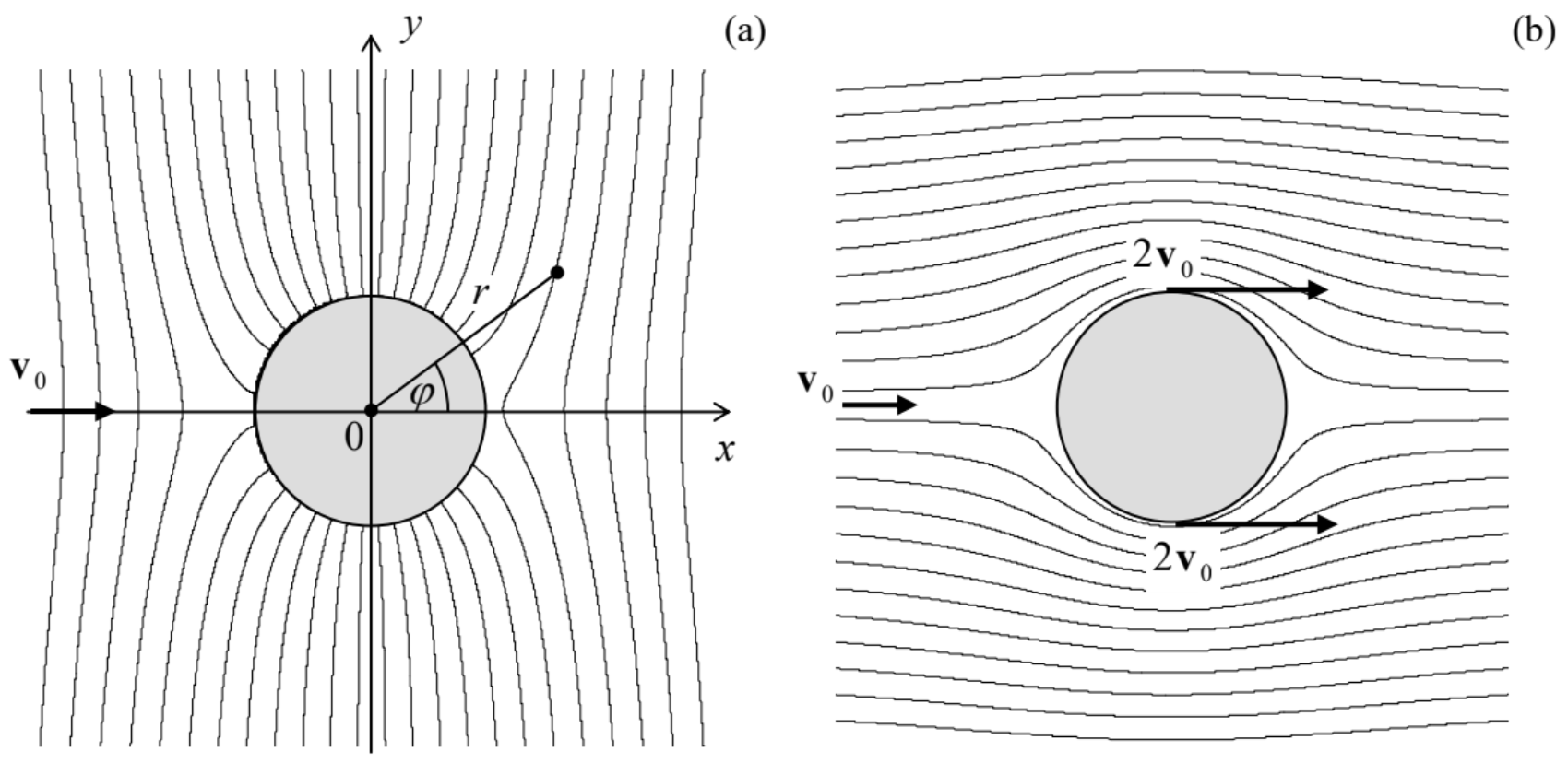Figure 8.8. The flow of an ideal, incompressible fluid around a cylinder: (a) equipotential surfaces and (b) streamlines.

Figure 8 a shows the surfaces of constant velocity potential \(\phi\) given by Eq. (37a). To find the fluid velocity, it is easier to rewrite that equality in the Cartesian coordinates \(x=\rho \cos \varphi, y=\rho \sin \varphi\) : \[\phi=-v_{0} x\left(1+\frac{R^{2}}{\rho^{2}}\right)=-v_{0} x\left(1+\frac{R^{2}}{x^{2}+y^{2}}\right) .\] From here, we may readily calculate the Cartesian components \(v_{x}=-\partial \phi / \partial x\) and \(v_{y}=-\partial \phi / \partial y\) of fluid’s velocity. Figure \(8 \mathrm{~b}\) shows the flow streamlines. (They may be found by integration of the evident equation \(d y / d x=v_{y}(x, y) / v_{x}(x, y)\). For our simple problem, this integration may be done analytically, giving \(y\left[1-R^{2} /\left(x^{2}+y^{2}\right)\right]=\) const, where the constant is specific for each streamline.) One can see that the largest potential gradient, and hence the maximum fluid’s speed, is achieved at the vertical diameter’s ends \((\rho=R, \varphi=\pm \pi / 2)\), where \[v=v_{x}=-\left.\frac{\partial \phi}{\partial x}\right|_{r=R \atop x=0}=2 v_{0} .\] Now the pressure distribution may be calculated by plugging Eq. (37) into the Bernoulli equation (27) with \(u(\mathbf{r})=0\). The result shows that the pressure reaches its maximum at the ends of the longitudinal diameter \(y=0\), while at the ends of the transverse diameter \(x=0\), where the velocity is largest, it is lower by \(2 \rho v_{0}{ }^{2}\). (Here \(\rho\) is the fluid density again - sorry for the notation jitters!) Note that the distributions of both the velocity and the pressure are symmetric with respect to the transverse axis \(x\) \(=0\), so that the fluid flow does not create any net drag force in its direction. It may be shown that this result, which stems from the conservation of the mechanical energy of an ideal fluid, remains valid for a solid body of arbitrary shape moving inside an infinite volume of an ideal fluid - the so-called D’Alambert paradox. However, if a body moves near an ideal fluid’s surface, its energy may be transformed into that of the surface waves, and the drag becomes possible.

Speaking about the surface waves: the description of such waves in a gravity field \({ }^{27}\) is one more classical problem of the ideal fluid dynamics. \({ }^{28}\) Let us consider an open surface of an ideal fluid of density \(\rho\) in a uniform gravity field \(\mathbf{f}=\rho \mathbf{g}=-\rho g \mathbf{n}_{y}\) - see Figure 9. If the wave amplitude \(A\) is sufficiently small, we can neglect the nonlinear term \((\mathbf{v} \cdot \nabla) \mathbf{v} \propto A^{2}\) in the Euler equation (23) in comparison with the first term, \(\partial \mathbf{v} / \partial t\), which is linear in \(A\). For a wave with frequency \(\omega\) and wave number \(k\), the particle’s velocity \(\mathbf{v}=d \mathbf{q} / d t\) is of the order of \(\omega A\), so that this approximation is legitimate if \(\omega^{2} A \gg k(\omega A)^{2}\), i.e. when \[k A<<1,\] i.e. when the wave’s amplitude \(A\) is much smaller than its wavelength \(\lambda=2 \pi / k\). Due to this assumption, we may neglect the fluid vorticity effects, and (for an incompressible fluid) again use the Laplace equation (29) for the wave’s analysis.

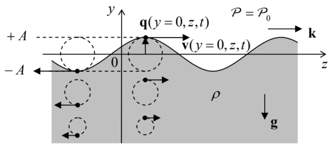
Figure 8.9. Small surface wave on a deep heavy fluid. Dashed lines show fluid particle trajectories. (For clarity, the displacement amplitude \(A\) is strongly exaggerated.)

Looking for its solution in the natural form of a sinusoidal wave, uniform in one of the horizontal directions \((x)\), \[\phi=\operatorname{Re}\left[\Phi(y) e^{i(k z-\omega t)}\right],\] we get a very simple equation \[\frac{d^{2} \Phi}{d y^{2}}-k^{2} \Phi=0,\] with an exponential solution (properly decaying at \(y \rightarrow-\infty), \Phi=\Phi_{A} \exp \{k y\}\), so that Eq. (40) becomes \[\phi=\operatorname{Re}\left[\Phi_{A} e^{k y} e^{i(k z-\omega t)}\right]=\Phi_{A} e^{k y} \cos (k z-\omega t),\] where the last form is valid if \(\Phi_{A}\) is real - which may be always arranged by a proper selection of the origins of \(z\) and/or \(t\). Note that the rate \(k\) of the wave’s decay in the vertical direction is exactly equal to the wave number of its propagation in the horizontal direction - along the fluid’s surface. Because of that, the trajectories of fluid particles are exactly circular - see Figure 9. Indeed, using Eqs. (28) and (42) to calculate velocity components, \[v_{x}=0, \quad v_{y}=-\frac{\partial \phi}{\partial y}=-k \Phi_{A} e^{k y} \cos (k z-\omega t), \quad v_{z}=-\frac{\partial \phi}{\partial z}=k \Phi_{A} e^{k y} \sin (k z-\omega t),\] we see that \(v_{y}\) and \(v_{z}\), at the same height \(y\), have equal real amplitudes, and are phase-shifted by \(\pi / 2\). This result becomes even more clear if we use the velocity definition \(\mathbf{v}=d \mathbf{q} / d t\) to integrate Eqs. (43) over time to recover the particle displacement law \(\mathbf{q}(t)\). Due to the strong inequality (39), the integration may be done at fixed \(y\) and \(z\) : \[q_{y}=q_{A} e^{k y} \sin (k z-\omega t), \quad q_{z}=q_{A} e^{k y} \cos (k z-\omega t), \quad \text { with } q_{A} \equiv \frac{k}{\omega} \Phi_{A} .\] Note that the phase of oscillations of \(v_{z}\) coincides with that of \(q_{y}\). This means, in particular, that at the wave’s "crest", particles are moving in the direction of the wave’s propagation - see arrows in Figure \(9 .\)

It is remarkable that all this picture follows from the Laplace equation alone! The "only" remaining feature to calculate is the dispersion law \(\omega(k)\), and for that, we need to combine Eq. (42) with what remains, in our linear approximation, of the Euler equation (23). In this approximation, and with the bulk force potential \(u=\rho g y\), the equation is reduced to \[\nabla\left(-\rho \frac{\partial \phi}{\partial t}+\mathcal{P}+\rho g y\right)=0 \text {. }\] This equality means that the function in the parentheses is constant in space; at the surface, and at negligible surface tension, it should be equal to the pressure \(\mathcal{P}_{0}\) above the surface (say, the atmospheric pressure), which we assume to be constant. This means that on the surface, the contributions to \(\mathcal{P}\) that come from the first and the third term in Eq. (45), should compensate each other. Let us take the average surface position for \(y=0\); then the surface with waves is described by the relation \(y(z, t)=q_{y}(y, z, t)-\) see Figure 9. Due to the strong relation (39), we can use Eqs. (42) and (44) with \(y=0\), so that the above compensation condition yields \[-\rho \omega \Phi_{A} \sin (k z-\omega t)+\rho g \frac{k}{\omega} \Phi_{A} \sin (k z-\omega t)=0 .\] This condition is identically satisfied on the whole surface (and for any \(\Phi_{A}\) ) as soon as \[\omega^{2}=g k,\] This equality is the dispersion relation we were looking for. Looking at this simple result (which includes just one constant, \(g\) ), note, first of all, that it does not involve the fluid’s density. This is not too surprising, because due to the weak equivalence principle, particle masses always drop out from the solutions of problems involving gravitational forces alone. Second, the dispersion law (47) is strongly nonlinear, and in particular does not have an acoustic wave limit at all. This means that the surface wave propagation is strongly dispersive, with both the phase velocity \(v_{\mathrm{ph}} \equiv \omega / k=g / \omega\) and the group velocity \(v_{\mathrm{gr}} \equiv d \omega / d k=g / 2 \omega \equiv v_{\mathrm{ph}} / 2\) diverging at \(\omega \rightarrow 0\).

This divergence is an artifact of our assumption of the infinitely thick fluid’s layer. A rather straightforward generalization of the above calculations to a layer of a finite thickness \(h\), using the additional boundary condition \(\left.v_{y}\right|_{y=h}=0\) (left for the reader’s exercise), yields a more general dispersion relation: \[\omega^{2}=g k \tanh k h .\] It shows that relatively long waves, with \(\lambda \gg h\), i.e. with \(k h \ll 1\), propagate without dispersion (i.e. have \(\omega / k=\) const \(\equiv v\) ), with the following velocity: \[v=(g h)^{1 / 2} .\] For the Earth’s oceans, this velocity is rather high, approaching \(300 \mathrm{~m} / \mathrm{s}(!)\) for \(h=10 \mathrm{~km}\). This result explains, in particular, the very fast propagation of tsunami waves.

In the opposite limit of very short waves (large \(k\) ), Eq. (47) also does not give a good description of experimental data, due to surface tension effects - see Sec. 2 above. Using Eq. (13), it is easy (and hence also left for the reader’s exercise) to show that their account leads (at \(k h>>1\) ) to the following modification of Eq. (47): \[\omega^{2}=g k+\frac{\not k^{3}}{\rho} .\] According to this formula, the surface tension is important at wavelengths smaller than the capillary constant \(a_{\mathrm{c}}\) given by Eq. (14). Much shorter waves, for that Eq. (50) yields \(\omega \propto k^{3 / 2}\), are called the capillary waves - or just "ripples".

---

\({ }^{16}\) It was derived in 1755 by the same Leonhard Euler whose name has already been (reverently) mentioned several times in this course.

\({ }^{17}\) It readily follows, for example, from MA Eq. (11.6) with \(\mathbf{g}=\mathbf{f}=\mathbf{v}\).

\({ }^{18}\) Named after Daniel Bernoulli (1700-1782), not to be confused with Jacob Bernoulli or one of several Johanns of the same famous Bernoulli family, which gave the world so many famous mathematicians and scientists.

\({ }^{19}\) Perhaps the most spectacular manifestation of the vorticity conservation is the famous toroidal vortex rings (see, e.g., a nice photo and a movie at https://en.Wikipedia.org/wiki/Vortex_ring), predicted in 1858 by \(\mathrm{H}\). von Helmholtz, and then demonstrated by P. Tait in a series of spectacular experiments with smoke in the air. The persistence of such a ring, once created, is only limited by the fluid’s viscosity - see the next section.

\({ }_{20}\) This theorem was first formulated (verbally) by Hermann von Helmholtz.

\({ }^{21}\) Its proof may be found, e.g., in Sec. 8 of L. Landau and E. Lifshitz, Fluid Mechanics, \(2^{\text {nd }}\) ed., ButterworthHeinemann, \(1987 .\)

\({ }^{22}\) This case is very important, because the motion of a solid body, with a constant velocity \(\mathbf{u}\), in the otherwise stationary fluid, gives exactly the same problem (with \(\mathbf{v}_{0}=-\mathbf{u}\) ), in a reference frame bound to the body.

\({ }^{23}\) See, e.g., EM Secs. 2.3-2.8.

\({ }^{24}\) See, e.g., MA Eq. (10.3).

\({ }^{25}\) Let me hope that the letter \(\rho\), used here to denote the magnitude of the \(2 \mathrm{D}\) radius-vector \(\boldsymbol{\rho}=\{x, y\}\), will not be confused with the fluid’s density - which does not participate in this boundary problem.

\({ }^{26}\) See, e.g., EM Eq. (2.112). Note that the most general solution of Eq. (32) also includes a term proportional to \(\varphi\), but this term should be zero for such a single-valued function as the velocity potential.

\({ }^{27}\) The alternative, historic term "gravity waves" for this phenomenon may nowadays lead to confusion with the relativistic effect of gravity waves - which may propagate in free space.

\({ }^{28}\) It was solved by Sir George Biddell Airy (1801-19892), of the Airy functions fame. (He was also a prominent astronomer and, in particular, established Greenwich as the prime meridian.)