
9.3: Chaos in Hamiltonian Systems


- Last updated
- Jan 29, 2022
- Save as PDF

( \newcommand{\kernel}{\mathrm{null}\,}\)
The last conclusion is of course valid for Hamiltonian systems, which are just a particular type of dynamic systems. However, one may wonder whether these systems, that feature at least one first integral of motion, H= const, and hence are more "ordered" than the systems discussed above, can exhibit chaos at all. The answer is yes because such systems still can have mechanisms for exponential growth of a small initial perturbation.
As the simplest way to show it, let us consider the so-called mathematical billiard, i.e. system with a ballistic particle (a "ball") moving freely by inertia on a horizontal plane surface ("table") limited by rigid impenetrable walls. In this idealized model of the usual game of billiards, the ball’s velocity v is conserved when it moves on the table, and when it runs into a wall, the ball is elastically reflected from it as from a mirror, 14 with the reversal of the sign of the normal velocity vn, and the conservation of the tangential velocity vτ, and hence without any loss of its kinetic (and hence the full) energy E=H=T=m2v2=m2(v2n+v2τ).
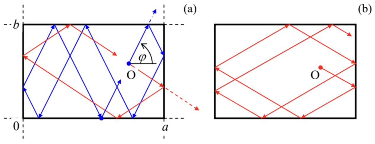 Figure 9.7. Ball motion on a rectangular billiard at (a) a commensurate, and (b) an incommensurate launch angle.
Such analysis (left for the reader’ pleasure :-) shows that if the tangent of the ball launching angle φ is commensurate with the side length ratio: tanφ=±mnba,
In 1963, i.e. well before E. Lorenz’s work, Yakov Sinai showed that the situation changes completely if an additional wall, in the shape of a circle, is inserted into the rectangular billiard (Figure 8). For most initial conditions, the ball’s trajectory eventually runs into the circle (see the red line on panel (a) as an example), and the further trajectory becomes essentially chaotic. Indeed, let us consider the ball’s reflection from the circle-shaped wall - Figure 8b. Due to the conservation of the tangential velocity, and the sign change of the normal velocity component, the reflection obeys a simple law: θr=θ1. Figure 8 b shows that as the result, the magnitude of a small difference δφ between the angles of two close trajectories (as measured in the lab system), doubles at each reflection from the curved wall. This means that the small deviation grows along the ball trajectory as |δφ(N)|∼|δφ(0)|×2N≡|δφ(0)|eNln2,
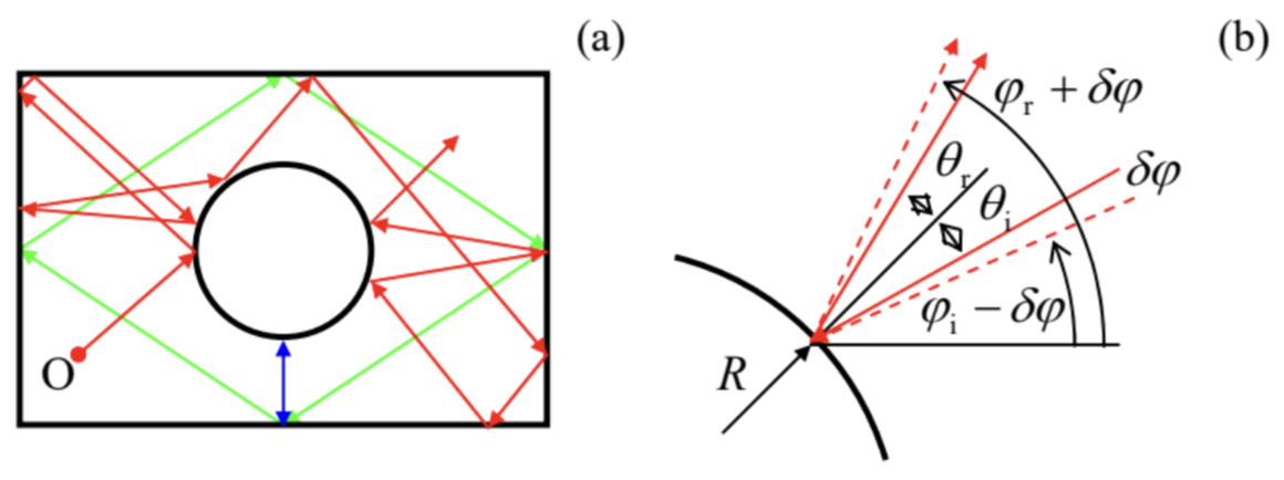 Figure 9.8. (a) Motion on a Sinai billiard table, and (b) the mechanism of the exponential divergence of close trajectories.
The most important new feature of the dynamic chaos in Hamiltonian systems is its dependence on initial conditions. (In the systems discussed in the previous two previous sections, that lack the integrals of motion, the initial conditions are rapidly "forgotten", and the chaos is usually characterized after an initial transient period - see, e.g., Figure 4.) Indeed, even a Sinai billiard allows periodic motion, along closed orbits, at certain initial conditions - see the blue and green lines in Figure 8a as examples. Thus the chaos "depth" in such systems may be characterized by the "fraction"18 of the phase space of initial parameters (for a 2D billiard, of the 3D space of initial values of x,y, and φ ) resulting in chaotic trajectories.
This conclusion is also valid for Hamiltonian systems that are met in experiment more frequently than the billiards, for example, coupled nonlinear oscillators without damping. Perhaps the earliest and the most popular example is the so-called Hénon-Heiles system, 19 which may be described by the following Lagrangian function: L=m12(˙q21−ω21q21)+m22(˙q22−ω22q22)−ε(q21−13q22)q2.
Let us start from the limit A1,2→0, when the oscillations of q2 are virtually sinusoidal. As we already know (see Figure 5.9 and its discussion), if the representation point highlighting was perfectly synchronous with frequency ω2 of the oscillations, there would be only one point on the Poincaré plane - see, e.g. the right top panel of Figure 4. However, at the q1 - initiated highlighting, there is not such synchronism, so that each period, a different point of the elliptical (at the proper scaling of the velocity, circular) trajectory is highlighted, so that the resulting points, for certain initial conditions, reside on a circle of radius A2. If we now vary the initial conditions, i.e. redistribute the initial energy between the oscillators, but keep the total energy E constant, on the Poincaré plane we get a set of ellipses.
Now, if the initial energy is increased, the nonlinear interaction of the oscillations starts to deform these ellipses, causing also their crossings - see, e.g., the top left panel of Figure 9. Still, below a certain threshold value of E, all Poincaré points belonging to a certain initial condition sit on a single closed contour. Moreover, these contours may be calculated approximately, but with pretty good accuracy, using straighforward generalization of the method discussed in Sec. 5.2.21
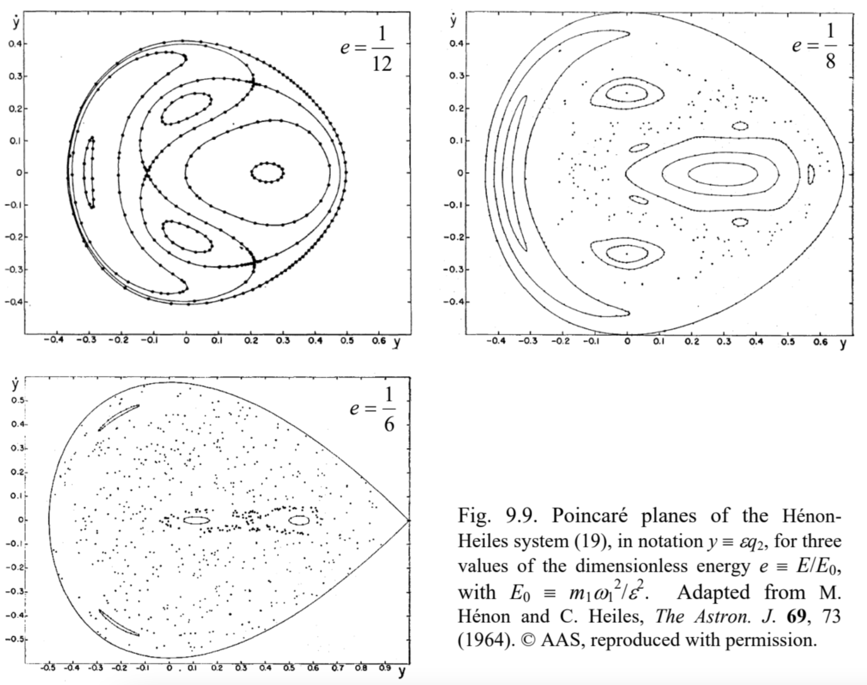
Figure 9.9. Poincaré planes of the HénonHeiles system (19), in notation y≡εq2, for three values of the dimensionless energy e≡E/E0, with E0≡m1ω12/ε2. Adapted from M. Hénon and C. Heiles, The Astron. J. 69,73 (1964). \odot AAS, reproduced with permission.
However, starting from some value of energy, certain initial conditions lead to sequences of points scattered over parts of the Poincaré plane, with a nonzero area - see the top right panel of Figure 9. This means that the corresponding oscillations q2(t) do not repeat from one (quasi-) period to the next one − cf. Figure 4 for the dissipative, forced pendulum. This is chaos. 22 However, some other initial conditions still lead to closed contours. This feature is similar to that in Sinai billiards, and is typical for Hamiltonian systems. As the energy is increased, larger and larger parts of the Poincaré plane correspond to the chaotic motion, signifying deeper and deeper chaos - see the bottom panel of Figure 9.
14 A more scientific-sounding name for such a reflection is specular-from the Latin word "speculum" meaning a metallic mirror.
15 Indeed, it is fully described by the following Lagrangian function: L=mv2/2−U(ρ), with U(ρ)=0 for the 2D radius vectors ρ belonging to the table area, and U(ρ)=+∞ outside the area.
16 Superficially, Eq. (17) is also valid for a plane wall, but as was discussed above, a billiard with such walls features a full correlation between sequential reflections, so that angle φ always returns to its initial value. In a Sinai billiard, such correlation disappears. Concave walls may also make a billiard chaotic; a famous example is the stadium billiard, suggested by Leonid Bunimovich in 1974, with two straight, parallel walls connecting two semi-circular, concave walls. Another example, which allows a straightforward analysis (first carried out by Martin Gutzwiller in the 1980s), is the so-called Hadamard billiard: an infinite (or rectangular) table with a nonhorizontal surface of negative curvature.
17 Curved-wall billiards are also a convenient platform for studies of quantum properties of classically chaotic systems (for their conceptual discussion, see QM Sec. 3.5), in particular, the features called "quantum scars" see, e.g., the spectacular numerical simulation results by E. Heller, Phys. Rev. Lett. 53,1515 (1984).
18 Actually, quantitative characterization of the fraction is not trivial, because it may have fractal dimensionality. Unfortunately, due to lack of time I have to refer the reader interested in this issue to special literature, e.g., the monograph by B. Mandelbrot (cited above) and references therein.
19 It was first studied in 1964 by Michel Hénon and Carl Heiles as a simple model of star rotation about a galactic center. Most studies of this equation have been carried out for the following particular case: m2=2m1,m1ω12= m2ω22. In this case, introducing new variables x≡εq1,y≡εq2, and τ≡ω1t, it is possible to rewrite Eqs. (18)-(20) in parameter-free forms. All the results shown in Figure 9 below are for this case.
20 Generally, the system has a trajectory in 4D space, e.g., that of coordinates q1,2 and their time derivatives, although the first integral of motion (20) means that for each fixed energy E, the motion is limited to a 3D subspace. Still, this is one dimension too many for a convenient representation of the motion.
21 See, e.g., M. Berry, in: S. Jorna (ed.), Topics in Nonlinear Dynamics, AIP Conf. Proc. No. 46, AIP, 1978, pp. 16-120.
22 This fact complies with the necessary condition of chaos, discussed at the end of Sec. 2 because Eqs. (19) may be rewritten as a system of four differential equations of the first order.