
14.4: The Hyperbola

( \newcommand{\kernel}{\mathrm{null}\,}\)
Cartesian Coordinates
The hyperbola has eccentricity e>1. In Cartesian coordinates, it has equation
x2a2−y2b2=1
and has two branches, both going to infinity approaching asymptotes x=±(a/b)y. The curve intersects the x axis at x=±a, the foci are at x=±ae for any point on the curve,
rF1−rF2=±2a
the sign being opposite for the two branches.
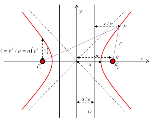
The semi-latus rectum, as for the earlier conics, is the perpendicular distance from a focus to the curve, and is ℓ=b2/a=a(e2−1). Each focus has an associated directrix, the distance of a point on the curve from the directrix multiplied by the eccentricity gives its distance from the focus.
Polar Coordinates
The (r,θ) equation with respect to a focus can be found by substituting x=rcosθ+ae,y=rsinθ in the Cartesian equation and solving the quadratic for u=1/r
Notice that θ has a limited range: the equation for the right-hand curve with respect to its own focus F2 has
tanθasymptote =±b/a, so cosθasymptote =±1/e
The equation for this curve is
ℓr=1−ecosθ
in the range
θasymptote <θ<2π−θasymptote
This equation comes up with various signs! The left hand curve, with respect to the left hand focus, would have a positive sign + e. With origin at F1 (on the left) the equation of the right-hand curve is ℓr=ecosθ−1 finally with the origin at F2 the left-hand curve is ℓr=−1−ecosθ. These last two describe repulsive inverse square scattering (Rutherford).
Note: A Useful Result for Rutherford Scattering
If we define the hyperbola by
x2a2−y2b2=1
then the perpendicular distance from a focus to an asymptote is just b.
This equation is the same (including scale) as
ℓ/r=−1−ecosθ, with ℓ=b2/a=a(e2−1)
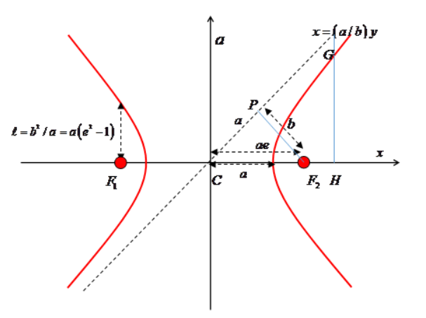
Proof: The triangle CPF2 is similar to triangle CHG, so PF2/PC=GH/CH=b/a and since the square of the hypotenuse CF2 is a2e2=a2+b2, the distance F2P=b
I find this a surprising result because in analyzing Rutherford scattering (and other scattering) the impact parameter, the distance of the ingoing particle path from a parallel line through the scattering center, is denoted by b. Surely this can’t be a coincidence? But I can’t find anywhere that this was the original motivation for the notation.