19.1: The Model

Notation! In this lecture, I use \(\kappa\) for the spring constant (\(k\) is a wave number) and \(\Omega\) for frequency (\(\omega\) is a root of unity).

A good classical model for a crystal is to represent the atoms by balls held in place by light springs, representing valence bonds, between nearest neighbors. The simplest such crystal that has some realistic features is a single chain of connected identical atoms. To make the math easy, we’ll connect the ends of the chain to make it a circle. This is called “imposing periodic boundary conditions”. It is common practice in condensed matter theory, and makes little difference to the physics for a large system.

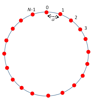
We’ll take the rest positions of the atoms to be uniformly spaced, a apart, with the first atom at a, the \(n^{\text {th }}\) atom at na, the final ​​​​\(N^{\text {th }}\) atom at the origin.

Away from the lowest energy state, we denote the position of the \(n^{\text {th }} \text { atom } n a+x_{n}\), so, as in our earlier discussion of oscillating systems, \(x_{n}\) is the displacement from equilibrium (which we take to be along the line—we are not considering transverse modes of vibration at this time).

The Lagrangian of this circular chain system is:

\[L=\sum_{n=1}^{N} \frac{1}{2} m \dot{x}_{n}^{2}-\sum_{n=1}^{N} \frac{1}{2} \kappa\left(x_{n+1}-x_{n}\right)^{2} \quad N+1 \equiv 1\]

We’re going to call the spring constant \(\kappa\), we’ll need \(k\) for something else. We’ll also call the frequency \(\Omega\)

Looking for eigenstates with frequency \(\Omega\), we find the set of equations

\[m \ddot{x}_{n}=-\kappa\left(2 x_{n}-x_{n-1}-x_{n+1}\right)\]

Taking a solution \(x_{n}=A_{n} e^{i \Omega t}\), with the understanding that \(A_{n}\) may be complex, and at the end \(x_{n}\) is just the real part of the formal solution, we find the eigenvalue equation for a chain of four atoms (the biggest Mathtype can handle!)

\begin{equation}
-m \Omega^{2}\left(\begin{array}{c}
A_{1} \\
A_{2} \\
A_{3} \\
A_{4}
\end{array}\right)=\left(\begin{array}{cccc}
-2 \kappa & \kappa & 0 & \kappa \\
\kappa & -2 \kappa & \kappa & 0 \\
0 & \kappa & -2 \kappa & \kappa \\
\kappa & 0 & \kappa & -2 \kappa
\end{array}\right)\left(\begin{array}{c}
A_{1} \\
A_{2} \\
A_{3} \\
A_{4}
\end{array}\right)
\end{equation}

Actually we’d have a much bigger matrix, with lots of zeroes, but hopefully the pattern is already clear: \(-2 \kappa\) or each diagonal element and \(\kappa\)’s in two diagonal-slanting lines flanking the main diagonal (corresponding to the links between nearest neighbors) and finally \(\kappa\)’s in the two far corners, these coming from the spring joining \(N to 1\) to complete the circle.

Notice first that if \(\Omega=0\) there is an eigenvector \((1,1,1,1)^{T}\), since the sum of the elements in one row is zero (the T means transpose, that is, it’s really a column vector, but row vectors are a lot easier to fit into the text here).

This eigenvector is just uniform displacement of the whole system, which costs zero energy since the system isn’t anchored to a particular place on the ring. We’ll assume, though, that the system as a whole is at rest, meaning the center of mass is stationary, and the atoms have well-defined rest positions as in the picture at \(a, 2 a, 3 a, \ldots, N a, N a \equiv 0\)