
4.2: Weak Nonlinearity


- Last updated
- Jun 28, 2021
- Save as PDF

( \newcommand{\kernel}{\mathrm{null}\,}\)
Most physical oscillators become non-linear with increase in amplitude of the oscillations. Consequences of non-linearity include breakdown of superposition, introduction of additional harmonics, and complicated chaotic motion that has great sensitivity to the initial conditions as illustrated in this chapter. Weak non-linearity is interesting since perturbation theory can be used to solve the non-linear equations of motion.
The potential energy function for a linear oscillator has a pure parabolic shape about the minimum location, that is, U=12k(x−x0)2 where x0 is the location of the minimum. Weak non-linear systems have small amplitude oscillations Δx about the minimum allowing use of the Taylor expansion
U(Δx)=U(x0)+ΔxdU(x0)dx+Δx22!d2U(x0)dx2+Δx33!d3U(x0)dx3+Δx44!d4U(x0)dx4+…
By definition, at the minimum dU(x0)dx=0, and thus Equation ??? can be written as
ΔU=U(Δx)−U(x0)=Δx22!d2U(x0)dx2+Δx33!d3U(x0)dx3+Δx44!d4U(x0)dx4+…
For small amplitude oscillations the system is linear when only the second-order Δx22!d2U(x0)dx2 term in Equation ??? is significant. The linearity for small amplitude oscillations greatly simplifies description of the oscillatory motion in that superposition applies, and complicated chaotic motion is avoided. For slightly larger amplitude motion, where the higher-order terms in the expansion are still much smaller than the second-order term, then perturbation theory can be used as illustrated by the simple plane pendulum which is non linear since the restoring force equals
mgsinθ≃mg(θ−θ33!+θ55!−θ77!+…)
This is linear only at very small angles where the higher-order terms in the expansion can be neglected. Consider the equation of motion at small amplitudes for the harmonically-driven, linearly-damped plane pendulum
¨θ+Γ˙θ+ω20sinθ=¨θ+Γ˙θ+ω20(θ−θ36)=F0cos(ωt)
where only the first two terms in the expansion ??? have been included. It was shown in chapter 3 that when sinθ≈θ then the steady-state solution of Equation ??? is of the form
θ(t)=Acos(ωt−δ)
Insert this first-order solution into Equation ???, then the cubic term in the expansion gives a term cos3ωt=14(cos3ωt+3cosωt). Thus the perturbation expansion to third order involves a solution of the form
θ(t)=Acos(ωt−δ)+Bcos3(ωt−δ)
This perturbation solution shows that the non-linear term has distorted the signal by addition of the third harmonic of the driving frequency with an amplitude that depends sensitively on θ. This illustrates that the superposition principle is not obeyed for this non-linear system, but, if the non-linearity is weak, perturbation theory can be used to derive the solution of a non-linear equation of motion.
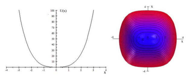
Figure 4.2.1 illustrates that for a potential U(x)=2x2+x4, the x4 non-linear term are greatest at the maximum amplitude x, which makes the total energy contours in state-space more rectangular than the elliptical shape for the harmonic oscillator as shown in figure (3.4.2). The solution is of the form given in Equation ???.
Example 4.2.1: Non-linear oscillator
Assume that a non-linear oscillator has a potential given by
U(x)=kx22−mλx33
where λ is small. Find the solution of the equation of motion to first order in λ, assuming x=0 at t=0.
Solution
The equation of motion for the nonlinear oscillator is
m¨x=−dUdx=−kx+mλx2
If the mλx2 term is neglected, then the second-order equation of motion reduces to a normal linear oscillator with
x0=Asin(ω0t+φ)
where
ω0=√km
Assume that the first-order solution has the form
x1=x0+λx1
Substituting this into the equation of motion, and neglecting terms of higher order than λ, gives
¨x1+ω20x1=x20=A22[1−cos(2ω0t)]
To solve this try a particular integral
x1=B+Ccos(2ω0t)
and substitute into the equation of motion gives
−3ω20Ccos(2ω0t)+ω20B=A22−A22cos(2ω0t)
Comparison of the coefficients gives
B=A22ω20C=A26ω20
The homogeneous equation is
¨x1+ω20x1=0
which has a solution of the form
x1=D1sin(ω0t)+D2cos(ω0t)
Thus combining the particular and homogeneous solutions gives
x1=(A+λD1)sin(ω0t)+λ[A22ω20+D2cos(ω0t)+A26ω20cos(2ω0t)]
The initial condition x=0 at t=0 then gives
D2=−2A23ω2
and
x1=(A+λD1)sin(ω0t)+λA2ω20[12−23cos(ω0t)+16cos(2ω0t)]
The constant (A+λD1) is given by the initial amplitude and velocity.
This system is nonlinear in that the output amplitude is not proportional to the input amplitude. Secondly, a large amplitude second harmonic component is introduced in the output waveform; that is, for a non-linear system the gain and frequency decomposition of the output differs from the input. Note that the frequency composition is amplitude dependent. This particular example of a nonlinear system does not exhibit chaos. The Laboratory for Laser Energetics uses nonlinear crystals to double the frequency of laser light.