
8.6: Routhian Reduction


- Last updated
- Mar 14, 2021
- Save as PDF

( \newcommand{\kernel}{\mathrm{null}\,}\)
Noether’s theorem states that if the coordinate qj is cyclic, and if the Lagrange multiplier plus generalized force contributions for the jth coordinates are zero, then the canonical momentum of the cyclic variable, pj, is a constant of motion as is discussed in chapter 7.3. Therefore, both (qj,pj) are constants of motion for cyclic variables, and these constant (qj,pj) coordinates can be factored out of the Hamiltonian H(p,q,t). This reduces the number of degrees of freedom included in the Hamiltonian. For this reason, cyclic variables are called ignorable variables in Hamiltonian mechanics. This advantage does not apply to the (qj,˙qj) variables used in Lagrangian mechanics since ˙q is not a constant of motion for a cyclic coordinate. The ability to eliminate the cyclic variables as unknowns in the Hamiltonian is a valuable advantage of Hamiltonian mechanics that is exploited extensively for solving problems, as is described in chapter 15.
It is advantageous to have the ability to exploit both the Lagrangian and Hamiltonian formulations simultaneously when handling systems that involve a mixture of cyclic and non-cyclic coordinates. The equations of motion for each independent generalized coordinate can be derived independently of the remaining generalized coordinates. Thus it is possible to select either the Hamiltonian or the Lagrangian formulations for each generalized coordinate, independent of what is used for the other generalized coordinates. Routh devised an elegant, and useful, hybrid technique that separates the cyclic and non-cyclic generalized coordinates in order to simultaneously exploit the differing advantages of both the Hamiltonian and Lagrangian formulations of classical mechanics. The Routhian reduction approach partitions the ∑ni=1pi˙qi kinetic energy term in the Hamiltonian into a cyclic group, plus a non-cyclic group, i.e.
H(q1,...,qn;p1,....,pn;t)=n∑i=1pi˙qi−L=s∑cyclicpi˙qi+n−s∑noncyclicpi˙qi−L
Routh’s clever idea was to define a new function, called the Routhian , that include only one of the two partitions of the kinetic energy terms. This makes the Routhian a Hamiltonian for the coordinates for which the kinetic energy terms are included, while the Routhian acts like a negative Lagrangian for the coordinates where the kinetic energy term is omitted. This book defines two Routhians.
Rcyclic(q1,...,qn;˙q1,...,˙qs;ps+1,....,pn;t)≡m∑cyclicpi˙qi−LRnoncyclic(q1,...,qn;p1,...,ps;˙qs+1,....,˙qn;t)≡s∑noncyclicpi˙qi−L
The first, Routhian, called Rcyclic, includes the kinetic energy terms only for the cyclic variables, and behaves like a Hamiltonian for the cyclic variables, and behaves like a Lagrangian for the non-cyclic variables. The second Routhian, called Rnon−cyclic, includes the kinetic energy terms for only the non-cyclic variables, and behaves like a Hamiltonian for the non-cyclic variables, and behaves like a negative Lagrangian for the cyclic variables. These two Routhians complement each other in that they make the Routhian either a Hamiltonian for the cyclic variables, or the converse where the Routhian is a Hamiltonian for the non-cyclic variables. The Routhians use (qi,˙qi) to denote those coordinates for which the Routhian behaves like a Lagrangian, and (qi,pi) for those coordinates where the Routhian behaves like a Hamiltonian. For uniformity, it is assumed that the degrees of freedom between 1≤i≤s are non-cyclic, while those between s+1≤i≤n are ignorable cyclic coordinates.
The Routhian is a hybrid of Lagrangian and Hamiltonian mechanics. Some textbooks minimize discussion of the Routhian on the grounds that this hybrid approach is not fundamental. However, the Routhian is used extensively in engineering in order to derive the equations of motion for rotating systems. In addition it is used when dealing with rotating nuclei in nuclear physics, rotating molecules in molecular physics, and rotating galaxies in astrophysics. The Routhian reduction technique provides a powerful way to calculate the intrinsic properties for a rotating system in the rotating frame of reference. The Routhian approach is included in this textbook because it plays an important role in practical applications of rotating systems, plus it nicely illustrates the relative advantages of the Lagrangian and Hamiltonian formulations in mechanics.
Rcyclic - Routhian is a Hamiltonian for the cyclic variables
The cyclic Routhian Rcyclic is defined assuming that the variables between 1≤i≤s are non-cyclic, where s=n−m, while the m variables between s+1≤i≤n are ignorable cyclic coordinates. The cyclic Routhian Rcyclic expresses the cyclic coordinates in terms of (q,p) which are required for use by Hamilton’s equations, while the non-cyclic variables are expressed in terms of (q,˙q) for use by the Lagrange equations. That is, the cyclic Routhian Rcyclic is defined to be
Rcyclic(q1,...,qn;˙q1,...,˙qs;ps+1,....,pn;t)≡m∑cyclicpi˙qi−L
where the summation ∑cyclicpi˙qi is over only the m cyclic variables s+1≤i≤n. Note that the Lagrangian can be split into the cyclic and the non-cyclic parts
Rcyclic(q1,...,qn;˙q1,...,˙qs;ps+1,....,pn;t)=m∑cyclicpi˙qi−Lcyclic−Lnoncyclic
The first two terms on the right can be combined to give the Hamiltonian Hcyclic for only the m cyclic variables, i=s+1,s+2,..,n, that is
Rcyclic(q1,...,qn;˙q1,...,˙qs;ps+1,....,pn;t)=Hcyclic−Lnoncyclic
The Routhian Rcyclic(q1,...,qn;˙q1,...,˙qs;ps+1,....,pn;t) also can be written in an alternate form
Rcyclic(q1,...,qn;˙q1,...,˙qs;ps+1,....,pn;t)≡m∑cyclicpi˙qi−L=n∑i=1pi˙qi−L−s∑noncyclicpi˙q=H−s∑noncyclicpi˙qi
which is expressed as the complete Hamiltonian minus the kinetic energy term for the noncyclic coordinates. The Routhian Rcyclic behaves like a Hamiltonian for the m cyclic coordinates and behaves like a negative Lagrangian Lnoncyclic for all the s=n−m noncyclic coordinates i=1,2,...,s. Thus the equations of motion for the s non-cyclic variables are given using Lagrange’s equations of motion, while the Routhian behaves like a Hamiltonian Hcyclic for the m ignorable cyclic variables i=s+1,...,n.
Ignoring both the Lagrange multiplier and generalized forces, then the partitioned equations of motion for the non-cyclic and cyclic generalized coordinates are given in Table 8.6.1.
| Lagrange equations | Hamilton equations | |
|---|---|---|
| Coordinates | Noncyclic: 1≤i≤s | Cyclic: (s+1)≤i≤n |
| ∂Rcyclic∂qi=−∂Lnoncyclic∂qi | ∂Rcyclic∂qi=−˙pi | |
| Equations of motion | ||
| ∂Rcyclic∂˙qi=−∂Lnoncyclic∂˙qi | ∂Rcyclic∂pi=˙qi |
Thus there are m cyclic (ignorable) coordinates (q,p)s+1,....,(q,p)n which obey Hamilton’s equations of motion, while the the first s=n−m non-cyclic (non-ignorable) coordinates (q,˙q)1,....,(q,˙q)s for i=1,2,...,s obey Lagrange equations. The solution for the cyclic variables is trivial since they are constants of motion and thus the Routhian Rcyclic has reduced the number of equations of motion that must be solved from n to the s=n−m non-cyclic variables. This Routhian provides an especially useful way to reduce the number of equations of motion for rotating systems.
Note that there are several definitions used to define the Routhian, for example some books define this Routhian as being the negative of the definition used here so that it corresponds to a positive Lagrangian. However, this sign usually cancels when deriving the equations of motion, thus the sign convention is unimportant if a consistent sign convention is used.
Rnoncyclic - Routhian is a Hamiltonian for the non-cyclic variables
The non-cyclic Routhian Rnoncyclic complements Rcyclic. Again the generalized coordinates between 1≤i≤s are assumed to be non-cyclic, while those between s+1≤i≤n are ignorable cyclic coordinates. However, the expression in terms of (q,p) and (q,˙q) are interchanged, that is, the cyclic variables are expressed in terms of (q,˙q) and the non-cyclic variables are expressed in terms of (q,p) which is opposite of what was used for Rcyclic.
Rnoncyclic(q1,...,qn;p1,...,ps;˙qs+1,....,˙qn;t)=s∑noncyclicpi˙qi−Lnoncyclic−Lcyclic=Hnoncyclic−Lcyclic
It can be written in a frequently used form
Rnoncyclic(q1,...,qn;p1,...,ps;˙qs+1,....,˙qn;t)≡s∑noncyclicpi˙qi−L=n∑i=1pi˙qi−L−m∑cyclicpi˙qi=H−m∑cyclicpi˙qi
This Routhian behaves like a Hamiltonian for the s non-cyclic variables which are expressed in terms of q and p appropriate for a Hamiltonian. This Routhian writes the m cyclic coordinates in terms of q, and ˙q, appropriate for a Lagrangian, which are treated assuming the Routhian Rcyclic is a negative Lagrangian for these cyclic variables as summarized in table 8.6.2.
| Hamilton equations | Lagrange equations | |
|---|---|---|
| Coordinates | Noncyclic: 1≤i≤s | Cyclic: (s+1)≤i≤n |
| ∂Rnoncyclic∂qi=−˙pi | ∂Rnoncyclic∂qi=−∂Lcyclic∂qi | |
| Equations of motion | ||
| ∂Rnoncyclic∂pi=˙qi | ∂Rnoncyclic∂˙qi=−∂Lcyclic∂˙qi |
This non-cyclic Routhian Rnoncyclic is especially useful since it equals the Hamiltonian for the non-cyclic variables, that is, the kinetic energy for motion of the cyclic variables has been removed. Note that since the cyclic variables are constants of motion, then Rnoncyclic is a constant of motion if H is a constant of motion. However, Rnoncyclic does not equal the total energy since the coordinate transformation is time dependent, that is, Rnoncyclic corresponds to the energy of the non-cyclic parts of the motion. For example, when used to describe rotational motion, Rnoncyclic corresponds to the energy in the non-inertial rotating body-fixed frame of reference. This is especially useful in treating rotating systems such as rotating galaxies, rotating machinery, molecules, or rotating strongly-deformed nuclei as discussed in chapter 12.9.
The Lagrangian and Hamiltonian are the fundamental algebraic approaches to classical mechanics. The Routhian reduction method is a valuable hybrid technique that exploits a trick to reduce the number of variables that have to be solved for complicated problems encountered in science and engineering. The Routhian Rnoncyclic provides the most useful approach for solving the equations of motion for rotating molecules, deformed nuclei, or astrophysical objects in that it gives the Hamiltonian in the non-inertial body-fixed rotating frame of reference ignoring the rotational energy of the frame. By contrast, the cyclic Routhian Rcyclic is especially useful to exploit Lagrangian mechanics for solving problems in rigid-body rotation such as the Tippe Top described in example 14.23.2.
Note that the Lagrangian, Hamiltonian, plus both the Rnoncyclic and Rnoncyclic Routhian’s, all are scalars under rotation, that is, they are rotationally invariant. However, they may be expressed in terms of the coordinates in either the stationary or a rotating frame. The major difference is that the Routhian includes only subsets of the kinetic energy term ∑jpj˙qj. The relative merits of using Lagrangian, Hamiltonian, and both the Rnoncyclic and Rnoncyclic Routhian reduction methods, are illustrated by the following examples.
Example 8.6.1: Spherical pendulum using Hamiltonian mechanics
The spherical pendulum provides a simple test case for comparison of the use of Lagrangian mechanics, Hamiltonian mechanics, and both approaches to Routhian reduction. The Lagrangian mechanics solution of the spherical pendulum is described in example 6.8.7. The solution using Hamiltonian mechanics is given in this example followed by solutions using both of the Routhian reduction approaches.
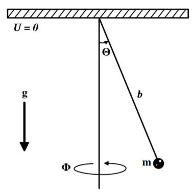
Consider the equations of motion of a spherical pendulum of mass m and length b. The generalized coordinates are θ,ϕ since the length is fixed at r=b. The kinetic energy is
T=12mb2.θ2+12mb2sin2θ.ϕ2
The potential energy U=−mgbcosθ giving that
L(r,θ,ϕ,˙r,˙θ,˙ϕ)=12mb2.θ2+12mb2sin2θ.ϕ2+mgbcosθ
The generalized momenta are
pθ=∂L∂˙θ=mb2.θpϕ=∂L∂˙ϕ=mb2sin2θ.ϕ
Since the system is conservative, and the transformation from rectangular to spherical coordinates does not depend explicitly on time, then the Hamiltonian is conserved and equals the total energy. The generalized momenta allow the Hamiltonian to be written as
H(r,θ,ϕ,pr,pθ,pϕ)=p2θ2mb2+p2ϕ2mb2sin2θ−mgbcosθ
The equations of motion are .˙pθ=−∂H∂θ=p2ϕcosθ2mb2sin3θ−mgbsinθ
˙pϕ=−∂H∂ϕ=0
˙θ=∂H∂pθ=pθmb2
˙ϕ=∂H∂pϕ=pϕmb2sin2θ Take the time derivative of Equation c and use a to substitute for ˙pθ gives that ¨θ−p2ϕcosθm2b4sin3θ+gbsinθ=0
Note that Equation b shows that ϕ is a cyclic coordinate. Thus
pϕ=mb2sin2θ˙ϕ=constant
that is the angular momentum about the vertical axis is conserved. Note that although pϕ is a constant of motion, ˙ϕ=pϕmb2sin2θ is a function of θ, and thus in general it is not conserved. There are various solutions depending on the initial conditions. If pϕ=0 then the pendulum is just the simple pendulum discussed previously that can oscillate, or rotate in the θ direction. The opposite extreme is where pθ=0 where the pendulum rotates in the ϕ direction with constant θ. In general the motion is a complicated coupling of the θ and ϕ motions.
Example 8.6.2: Spherical pendulum using Rcyclic(r,θ,ϕ,˙r,˙θ,pϕ)
The Lagrangian for the spherical pendulum is
L(r,θ,ϕ,˙r,˙θ,˙ϕ)=12mb2˙θ2+12mb2sin2θ˙ϕ2+mgbcosθ
Note that the Lagrangian is independent of ϕ, therefore ϕ is an ignorable variable with
˙pϕ=∂L∂ϕ=−∂H∂ϕ=0
Therefore pϕ is a constant of motion equal to
pϕ=∂L∂˙ϕ=mb2sin2θ˙ϕ
The Routhian Rcyclic(r,θ,ϕ,˙r,˙θ,pϕ) equals
Rcyclic(r,θ,ϕ,˙r,˙θ,pϕ)=pϕ˙ϕ−L=−[12mb2˙θ2+12mb2sin2θ˙ϕ2+mgbcosθ−mb2sin2θ˙ϕ2]=−12mb2˙θ2+12p2ϕmb2sin2θ+mgbcosθ
The Routhian Rcyclic(r,θ,ϕ,˙r,˙θ,pϕ) behaves like a Hamiltonian for ϕ, and like a Lagrangian L′=−Rcyclic for θ. Use of Hamilton’s canonical equations for ϕ give
˙ϕ=∂Rcyclic∂pϕ=pϕmb2sin2θ−˙pϕ=∂Rcyclic∂ϕ=0
These two equations show that pϕ is a constant of motion given by mb2sin2θ˙ϕ=pϕ= constant
Note that the Hamiltonian only includes the kinetic energy for the ϕ motion which is a constant of motion, but this energy does not equal the total energy. This solution is what is predicted by Noether’s theorem due to the symmetry of the Lagrangian about the vertical ϕ axis.
Since Rcyclic(r,θ,ϕ,˙r,˙θ,pϕ) behaves like a Lagrangian for θ then the Lagrange equation for θ is
ΛθL=ddt∂Rcyclic∂˙θ−∂Rcyclic∂θ=0
where the negative sign of the Lagrangian in Rcyclic(r,θ,ϕ,˙r,˙θ,pϕ) cancels. This leads to
mb2¨θ=p2ϕcosθmb2sin3θ−mgbsinθ
that is ¨θ−p2ϕcosθm2b4sin3θ+gbsinθ=0
This result is identical to the one obtained using Lagrangian mechanics in example 7.8.7 and Hamiltonian mechanics given in example 8.6.1. The Routhian Rcyclic simplified the problem to one degree of freedom θ by absorbing into the Hamiltonian the ignorable cyclic ϕ coordinate and its conserved conjugate momentum pϕ. Note that the central term in Equation β is the centrifugal term which is due to rotation about the vertical axis. This term is zero for plane pendulum motion when pϕ=0.
Example 8.6.3: Spherical pendulum using Rnoncyclic(r,θ,pr,pθ,˙ϕ)
For a rotational system the Routhian Rnoncyclic(r,θ,ϕ,pr,pθ,˙ϕ) also can be used to project out the Hamiltonian for the active variables in the rotating body-fixed frame of reference. Consider the spherical pendulum where the rotating frame is rotating with angular velocity ˙ϕ. The Lagrangian for the spherical pendulum is
L(r,θ,ϕ,˙r,˙θ,˙ϕ)=12mb2˙θ2+12mb2sin2θ˙ϕ2+mgbcosθ
Note that the Lagrangian is independent of ϕ, therefore ϕ is an ignorable variable with
˙pϕ=∂L∂ϕ=−∂H∂ϕ=0
Therefore pϕ is a constant of motion equal to
pϕ=∂L∂˙ϕ=mb2sin2θ˙ϕ
The total Hamiltonian is given by
H(r,θ,ϕ,pr,pθ,pϕ)=∑ipi˙qi−L=p2θ2mb2+p2ϕ2mb2sin2θ−mgbcosθ The Routhian for the rotating frame of reference Hrot is given by Equation 8.6.14, that is
Rnoncyclic(r,θ,ϕ,pr,pθ,˙ϕ)=n∑i=1pi˙qi−pϕ˙ϕ−L=H−pϕ˙ϕ=p2θ2mb2+p2ϕ2mb2sin2θ−mgbcosθ−pϕ˙ϕ=p2θ2mb2−12mb2sin2θ˙ϕ2−mgbcosθ
This behaves like a negative Lagrangian for ϕ and a Hamiltonian for θ. The conjugate momenta are
pϕ=∂L∂˙ϕ=−∂Rnoncyclic∂˙ϕ=mb2sin2θ˙ϕ˙pϕ=∂L∂ϕ=−∂Rnoncyclic∂ϕ=0
that is, pϕ is a constant of motion.
Hamilton’s equations of motion give
˙θ=∂Rnoncyclic∂pθ=pθmb2−˙pθ=∂Rnoncyclic∂θ=−p2ϕcosθmb2sin3θ+mgbsinθ
Equation δ gives that
∂∂t˙θ=¨θ=˙pθmb2
Inserting this into Equation ϵ gives
¨θ−p2ϕcosθm2b4sin3θ+gbsinθ=0
which is identical to the equation of motion α derived using Rcyclic. The Hamiltonian in the rotating frame is a constant of motion given by γ, but it does not include the total energy.
Note that these examples show that both forms of the Routhian, as well as the complete Lagrangian formalism, shown in example 7.8.7, and complete Hamiltonian formalism, shown in example 8.6.1, all give the same equations of motion. This illustrates that the Lagrangian, Hamiltonian, and Routhian mechanics all give the same equations of motion and this applies both in the static inertial frame as well as a rotating frame since the Lagrangian, Hamiltonian and Routhian all are scalars under rotation, that is, they are rotationally invariant.
Example 8.6.4: Single particle moving in a vertical plane under the influence of an inverse-square central force
The Lagrangian for a single particle of mass m, moving in a vertical plane and subject to a central inverse square central force, is specified by two generalized coordinates, r, and θ.
L=m2(˙r2+r2˙θ2)+kr
The ignorable coordinate is θ, since it is cyclic. Let the constant conjugate momentum be denoted by pθ=∂L∂˙θ=mr2˙θ. Then the corresponding cyclic Routhian is
Rcyclic(r,θ,˙r,pθ)=pθ˙θ−L=p2θ2mr2−12m˙r2−kr
This Routhian is the equivalent one-dimensional potential U(r) minus the kinetic energy of radial motion.
Applying Hamilton’s equation to the cyclic coordinate θ gives
˙pθ=0pθmr2=˙θ
implying a solution
pθ=mr2˙θ=l
where the angular momentum l is a constant.
The Lagrange-Euler equation can be applied to the non-cyclic coordinate r
ΛrL=ddt∂Rcyclic∂˙r−∂Rcyclic∂r=0 where the negative sign of Rcyclic cancels. This leads to the radial solution
m¨r−p2θmr3+kr2=0
where pθ=l which is a constant of motion in the centrifugal term. Thus the problem has been reduced to a one-dimensional problem in radius r that is in a rotating frame of reference.