19.4: Appendix - Orthogonal Coordinate Systems

The methods of vector analysis provide a convenient representation of physical laws. However, the manipulation of scalar and vector fields is greatly facilitated by use of components with respect to an orthogonal coordinate system such as the following.

Cartesian coordinates \((x, y, z)\)

Cartesian coordinates (rectangular) provide the simplest orthogonal rectangular coordinate system. The unit vectors specifying the direction along the three orthogonal axes are taken to be \((\mathbf{\hat{i}},\mathbf{\hat{j}}, \mathbf{\hat{k}})\). In cartesian coordinates scalar and vector functions are written as

\[\phi = \phi (x, y, z) \label{C.1}\]

\[\mathbf{r} = x\mathbf{\hat{i}}+y\mathbf{\hat{j}}+z\mathbf{\hat{k}} \label{C.2}\]

Calculation of the time derivatives of the position vector is especially simple using cartesian coordinates because the unit vectors \((\mathbf{\hat{i}},\mathbf{\hat{j}}, \mathbf{\hat{k}})\) are constant and independent in time. That is;

\[\frac{d\mathbf{\hat{i}}}{ dt} = \frac{d\mathbf{\hat{j}}}{ dt} = \frac{d\mathbf{\hat{k}}}{ dt} = 0 \nonumber\]

Since the time derivatives of the unit vectors are all zero then the velocity \(\mathbf{\dot{r}} = \frac{d\mathbf{r}}{ dt}\) reduces to the partial time derivatives of \(x\), \(y\), and \(z\). That is,

\[\mathbf{\dot{r}} = \dot{x} \mathbf{\hat{i}} + \dot{y} \mathbf{\hat{j}} + \dot{z} \mathbf{\hat{k}} \label{C.3}\]

Similarly the acceleration is given by

\[\mathbf{\ddot{r}} = \ddot{x} \mathbf{\hat{i}} + \ddot{y} \mathbf{\hat{j}} + \ddot{z} \mathbf{\hat{k}} \label{C.4}\]

Curvilinear coordinate systems

There are many examples in physics where the symmetry of the problem makes it more convenient to solve motion at a point \(P(x, y, z)\) using non-cartesian curvilinear coordinate systems. For example, problems having spherical symmetry are most conveniently handled using a spherical coordinate system \((r, \theta , \phi )\) with the origin at the center of spherical symmetry. Such problems occur frequently in electrostatics and gravitation; e.g. solutions of the atom, or planetary systems. Note that a cartesian coordinate system still is required to define the origin plus the polar and azimuthal angles \(\theta , \phi \). Using spherical coordinates for a spherically symmetry system allows the problem to be factored into a cyclic angular part, the solution which involves spherical harmonics that are common to all such spherically-symmetric problems, plus a one-dimensional radial part that contains the specifics of the particular spherically-symmetric potential. Similarly, for problems involving cylindrical symmetry, it is much more convenient to use a cylindrical coordinate system \((\rho , \phi , z)\). Again it is necessary to use a cartesian coordinate system to define the origin and angle \(\phi \). Motion in a plane can be handled using two dimensional polar coordinates.

Curvilinear coordinate systems introduce a complication in that the unit vectors are time dependent in contrast to cartesian coordinate system where the unit vectors \((\mathbf{\hat{i}},\mathbf{\hat{j}}, \mathbf{\hat{k}})\) are independent and constant in time. The introduction of this time dependence warrants further discussion.

Each of the three axes \(q_i\) in curvilinear coordinate systems can be expressed in cartesian coordinates \((x, y, z)\) as surfaces of constant \(q_i\) given by the function

\[q_i = f_i (x, y, z) \label{C.5}\]

where \(i = 1\), \(2\), or \(3\). An element of length \(ds_i\) perpendicular to the surface \(q_i\) is the distance between the surfaces \(q_i\) and \(q_i + dq_i\) which can be expressed as

\[ds_i = h_idq_i \label{C.6}\]

where \(h_i\) is a function of \((q_1, q_2, q_3)\). In cartesian coordinates \(h_1\), \(h_2\), and \(h_3\) are all unity. The unit-length vectors \(\hat{q}_1\), \(\hat{q}_2\), \(\hat{q}_3\), are perpendicular to the respective \(q_1\), \(q_2\), \(q_3\) surfaces, and are oriented to have increasing indices such that \(\mathbf{\hat{q}}_1 \times \mathbf{\hat{q}}_2 = \mathbf{\hat{q}}_3\). The correspondence of the curvilinear coordinates, unit vectors, and transform coefficients to cartesian, polar, cylindrical and spherical coordinates is given in Table \(\PageIndex{1}\).

Table \(\PageIndex{1}\): Curvilinear coordinates

Curvilinear	\(q_1\)	\(q_2\)	\(q_3\)	\(\mathbf{\hat{q}}_1\)	\(\mathbf{\hat{q}}_2\)	\(\mathbf{\hat{q}}_3\)	\(h_1\)	\(h_2\)	\(h_3\)
Cartesian	\(x\)	\(y\)	\(z\)	\(\hat{i}\)	\(\hat{j}\)	\(\mathbf{\hat{k}}\)	1	1	1
Polar	\(r\)	\(\theta\)		\(\mathbf{\hat{r}}\)	\(\boldsymbol{\hat{\theta}}\)		1	\(r\)
Cylindrical	\(\rho\)	\(\varphi\)	\(z\)	\(\boldsymbol{\hat{\rho}}\)	\(\boldsymbol{\hat{\varphi}}\)	\(\mathbf{\hat{z}}\)	1	\(\rho\)	1
Spherical	\(r\)	\(\theta\)	\(\varphi\)	\(\mathbf{\hat{r}}\)	\(\boldsymbol{\hat{\theta}}\)	\(\boldsymbol{\hat{\varphi}}\)	1	\(r\)	\(r\sin\theta\)

The differential distance and volume elements are given by

\[d\mathbf{s} = ds_1\mathbf{\hat{q}}_1 + ds_2\mathbf{\hat{q}}_2 + ds_3\mathbf{\hat{q}}_3 = h_1dq_1\mathbf{\hat{q}}_1 + h_2dq_2\mathbf{\hat{q}}_2 + h_3dq_3\mathbf{\hat{q}}_3 \label{C.7}\]

\[d \tau = ds_1ds_2ds_3 = h_1h_2h_3(dq_1dq_2dq_3) \label{C.8}\]

These are evaluated below for polar, cylindrical, and spherical coordinates.

Two-dimensional polar coordinates \((r, \theta )\)

The complication and implications of time-dependent unit vectors are best illustrated by considering twodimensional polar coordinates which is the simplest curvilinear coordinate system. Polar coordinates are a special case of cylindrical coordinates, when \(z\) is held fixed, or a special case of spherical coordinate system, when \(\phi\) is held fixed.

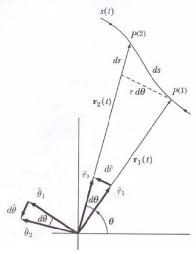
Consider the motion of a point \(P\) as it moves along a curve \(\mathbf{s}(t)\) such that in the time interval \(dt\) it moves from \(P^{(1)}\) to \(P^{(2)}\) as shown in Figure \(\PageIndex{1}\). The two-dimensional polar coordinates have unit vectors \(\mathbf{\hat{r}}, \boldsymbol{\hat{\theta}}\), which are orthogonal and change from \(\mathbf{\hat{r}}_1, \boldsymbol{\hat{\theta}}_1\), to \(\mathbf{\hat{r}}_2, \boldsymbol{\hat{\theta}}_2\), in the time \(dt\). Note that for these polar coordinates the angle unit vector \(\boldsymbol{\hat{\theta}}\) is taken to be tangential to the rotation since this is the direction of motion of a point on the circumference at radius \(r\).

The net changes shown in figure of Table \(\PageIndex{2}\) are

\[d\mathbf{\hat{r}} = \mathbf{\hat{r}}_2 − \mathbf{\hat{r}}_1 = d\mathbf{\hat{r}} = |\mathbf{\hat{r}}| d\theta \boldsymbol{\hat{\theta}} =d\theta \boldsymbol{\hat{\theta}} \label{C.9}\]

since the unit vector \(\mathbf{\hat{r}}\) is a constant with \(|\mathbf{\hat{r}}| = 1\). Note that the infinitessimal \(d\mathbf{\hat{r}}\) is perpendicular to the unit vector \(\mathbf{\hat{r}}\), that is, \(d\mathbf{\hat{r}}\) points in the tangential direction \(\boldsymbol{\hat{\theta}}\).

Similarly, the infinitessimal

\[d\boldsymbol{\hat{\theta}} = \boldsymbol{\hat{\theta}}_2 − \boldsymbol{\hat{\theta}}_1 = d\boldsymbol{\hat{\theta}} = −d\theta \mathbf{\hat{r}} \label{C.10}\]

which is perpendicular to the tangential \(\boldsymbol{\hat{\theta}}\) unit vector and therefore points in the direction \(−\mathbf{\hat{r}} \). The minus sign causes \(−d\theta \mathbf{\hat{r}}\) to be directed in the opposite direction to \(\mathbf{\hat{r}}\).

The net distance element \(d\mathbf{s}\) is given by

\[d\mathbf{s} =dr\mathbf{\hat{r}} + rd\mathbf{\hat{r}} =dr\mathbf{\hat{r}} + rd\theta \boldsymbol{\hat{\theta}} \label{C.11}\]

This agrees with the prediction obtained using Table \(\PageIndex{1}\).

The time derivatives of the unit vectors are given by equations \ref{C.9} and \ref{C.10} to be,

\[\frac{d\mathbf{\hat{r}}}{ dt} = \frac{d\theta}{ dt} \boldsymbol{\hat{\theta}} \label{C.12}\]

\[\frac{d\boldsymbol{\hat{\theta}}}{ dt} = −\frac{d\theta}{ dt} \mathbf{\hat{r}} \label{C.13}\]

Note that the time derivatives of unit vectors are perpendicular to the corresponding unit vector, and the unit vectors are coupled.

Consider that the velocity \(\mathbf{v}\) is expressed as

\[\mathbf{v} = \frac{d\mathbf{r}}{ dt} = \frac{d}{ dt}(r\mathbf{\hat{r}}) = \frac{dr}{ dt}\mathbf{\hat{r}} + r \frac{d\mathbf{\hat{r}} }{dt} = \dot{r}\mathbf{\hat{r}} + r \dot{\theta} \boldsymbol{\hat{\theta}} \label{C.14}\]

The velocity is resolved into a radial component \(\dot{r}\) and an angular, transverse, component \(r \dot{\theta} \).

Similarly the acceleration is given by

\[\mathbf{a} = \frac{d\mathbf{v}}{ dt} = \frac{d\dot{r} }{dt} \mathbf{\hat{r}}+\dot{r} \frac{d\mathbf{\hat{r}}}{ dt} + \frac{dr}{ dt} \dot{\theta} \boldsymbol{\hat{\theta}}+ r \frac{d\dot{\theta} }{dt} \boldsymbol{\hat{\theta}}+r \dot{\theta} \frac{d\boldsymbol{\hat{\theta}}}{ dt} \\ = \left( \ddot{r}− r \dot{\theta}^2\right) \mathbf{\hat{r}} + \left( \ddot{r}\theta + 2\dot{r} \dot{\theta} \right) \boldsymbol{\hat{\theta}} \label{C.15}\]

where the \(r \dot{\theta}^2 \mathbf{\hat{r}}\) term is the effective centripetal acceleration while the \(2\dot{r} \dot{\theta} \boldsymbol{\hat{\theta}}\) term is called the Coriolis term. For the case when \(\dot{r} = \ddot{r} = 0\), then the first bracket in \ref{C.15} is the centripetal acceleration while the second bracket is the tangential acceleration.

This discussion has shown that in contrast to the time independence of the cartesian unit basis vectors, the unit basis vectors for curvilinear coordinates are time dependent which leads to components of the velocity and acceleration involving coupled coordinates.

Table \(\PageIndex{2}\): Differential relations plus a diagram of the unit vectors for 2-dimensional polar coordinates.

Coordinates	\(r, \theta\)
Distance element	\(d\mathbf{s} = dr\mathbf{\hat{r}} + rd\theta \boldsymbol{\hat{\theta}}\)
Area element	\(da = r dr d\theta\)
Unit vectors	\(\mathbf{\hat{r}} = \hat{i} \cos \theta + \hat{j} \sin \theta\) \(\boldsymbol{\hat{\theta}} = -\hat{i} \sin \theta + \hat{j} \cos \theta\)
Time derivatives of unit vectors	\(\frac{d\mathbf{\hat{r}}}{dt} = \dot{\theta} \boldsymbol{\hat{\theta}}\) \(\frac{d\boldsymbol{\hat{\theta}}}{dt} = -\dot{\theta} \mathbf{\hat{r}} \)
Velocity	\(\mathbf{v} = \dot{r}\mathbf{\hat{r}} + r\dot{\theta} \boldsymbol{\hat{\theta}}\)
Kinetic energy	\(\frac{m}{2} \left(\dot{r}^2 + r^2 \dot{\theta}^2\right)\)
Acceleration	\(\mathbf{a} = \left(\ddot{r} - r \dot{\theta}^2\right)\mathbf{\hat{r}} + \left(r\ddot{\theta} + 2\dot{r}\dot{\theta}\right) \boldsymbol{\hat{\theta}}\)

Figure \(\PageIndex{1}\): Diagram for Table \(\PageIndex{2}\).

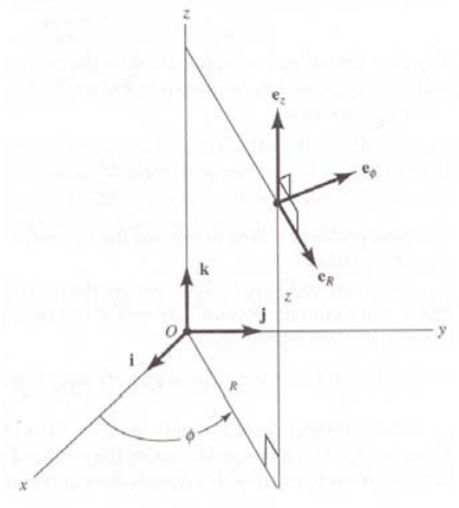
Cylindrical Coordinates \((\rho , \phi , z)\)

The three-dimensional cylindrical coordinates \((\rho , \phi , z)\) are obtained by adding the motion along the symmetry axis \(\mathbf{\hat{z}}\) to the case for polar coordinates. The unit basis vectors are shown in Table \(\PageIndex{3}\) where the angular unit vector \(\boldsymbol{\hat{\phi}}\) is taken to be tangential corresponding to the direction a point on the circumference would move. The distance and volume elements, the cartesian coordinate components of the cylindrical unit basis vectors, and the unit vector time derivatives are shown in Table \(\PageIndex{3}\). The time dependence of the unit vectors is used to derive the acceleration. As for the two-dimensional polar coordinates, the \(\boldsymbol{\hat{\rho}}\) and \(\boldsymbol{\hat{\theta}}\) direction components of the acceleration for cylindrical coordinates are coupled functions of \(\rho \), \(\dot{\rho}\), \(\ddot{\rho} \), \(\dot{\phi}\), and \(\ddot{\phi}\).

Table \(\PageIndex{3}\): Differential relations plus a diagram of the unit vectors for cylindrical coordinates.

Coordinates	\(\rho, \phi, \theta\)
Distance element	\(d\mathbf{s} = d \rho \boldsymbol{\hat{\rho}} + \rho d\phi \boldsymbol{\hat{\phi}} + dz\mathbf{\hat{z}}\)
Volume element	\(dv = \rho d\rho d\phi dz\)
Unit vectors	\(\boldsymbol{\hat{\rho}} = \hat{i} \cos \phi + \hat{j} \sin \phi\) \(\boldsymbol{\hat{\phi}} = -\hat{i} \sin \phi + \hat{j} \cos \phi\) \(\mathbf{\hat{z}} = \mathbf{\hat{k}}\)
Time derivatives of unit vectors	\(\frac{d\boldsymbol{\hat{\rho}}}{dt} = \dot{\phi} \boldsymbol{\hat{\phi}} \) \(\frac{d\boldsymbol{\hat{\phi}}}{dt} = -\dot{\phi} \boldsymbol{\hat{\rho}} \) \(\frac{d\mathbf{\hat{z}}}{dt} = 0\)
Velocity	\(\mathbf{v} = \dot{\rho} \boldsymbol{\hat{\rho}} + \rho \dot{\phi} \boldsymbol{\hat{\phi}} + \dot{z} \mathbf{\hat{z}}\)
Kinetic energy	\(\frac{m}{2} \left(\dot{\rho}^2 + \rho^2 \dot{\phi}^2 + \dot{z}^2 \right)\)
Acceleration	\(\mathbf{a} = \left(\ddot{\rho} - \rho \dot{\phi}^2\right)\boldsymbol{\hat{\rho}} + \left(\rho\ddot{\phi} + 2\dot{\rho}\dot{\phi}\right) \boldsymbol{\hat{\phi}} + \ddot{z}\mathbf{\hat{z}}\)

Figure \(\PageIndex{2}\): Diagram for Table \(\PageIndex{3}\).

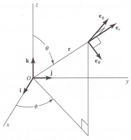
Spherical Coordinates \((r, \theta , \phi )\)

The three dimensional spherical coordinates, can be treated the same way as for cylindrical coordinates. The unit basis vectors are shown in Table \(\PageIndex{4}\) where the angular unit vectors \(\boldsymbol{\hat{\theta}}\) and \(\boldsymbol{\hat{\phi}}\) are taken to be tangential corresponding to the direction a point on the circumference moves for a positive rotation angle.

Table \(\PageIndex{4}\): Differential relations plus a diagram of the unit vectors for spherical coordinates.

Coordinates	\(r, \theta, \phi \)
Distance element	\(ds = dr\mathbf{\hat{r}} + rd\theta \boldsymbol{\hat{\theta}} + r \sin \theta d \phi \boldsymbol{\hat{\phi}}\)
Volume element	\(dv = r^2 \sin \theta drd\theta d\phi\)
Unit vectors	\(\mathbf{\hat{r}} = \hat{i} \sin \theta \cos \phi + \hat{j} \sin \theta \cos \phi + \mathbf{\hat{k}} \cos \theta\) \(\boldsymbol{\hat{\theta}} = \hat{i} \cos \theta \cos \phi + \hat{j} \cos \theta \sin \phi - \mathbf{\hat{k}} \sin \theta\) \(\boldsymbol{\hat{\phi}} = -\hat{i} \sin \phi + \hat{j} \cos \phi\)
Time derivatives of unit vectors	\(\frac{d\mathbf{\hat{r}}}{dt} = \boldsymbol{\hat{\theta}} \dot{\theta} + \boldsymbol{\hat{\phi}} \dot{\phi} \sin \theta \) \(\frac{d\boldsymbol{\hat{\theta}}}{dt} = -\mathbf{\hat{r}} \dot{\theta} + \boldsymbol{\hat{\phi}} \dot{\phi} \cos \theta \) \(\frac{d\boldsymbol{\hat{\phi}}}{dt} = -\mathbf{\hat{r}}\dot{\phi}\sin \theta - \boldsymbol{\hat{\theta}} \dot{\phi} \cos \theta \)
Velocity	\(\mathbf{v} = \dot{r}\mathbf{\hat{r}} + r\dot{\theta} \boldsymbol{\hat{\theta}} + r \dot{\phi} \sin \theta \boldsymbol{\hat{\phi}}\)
Kinetic energy	\(\frac{m}{2} \left(\dot{r}^2 + r^2 \dot{\theta}^2 + r^2\sin^2 \theta \dot{\phi}^2 \right)\)
Acceleration	\(\mathbf{a} = \left(\ddot{r} - r \dot{\theta}^2 - r\dot{\phi}^2 \sin^2 \theta \right)\mathbf{\hat{r}} + \left(r\ddot{\theta} + 2\dot{r}\dot{\theta} - r\dot{\phi}^2 \sin \theta \cos \theta \right) \boldsymbol{\hat{\theta}} + \left(r \ddot{\phi} \sin \theta + 2\dot{r}\dot{\phi} \sin \theta + 2r\dot{\theta}\dot{\phi} \cos \theta \right) \boldsymbol{\hat{\phi}} \)

Figure \(\PageIndex{3}\): Diagram for Table \(\PageIndex{4}\).

The distance and volume elements, the cartesian coordinate components of the spherical unit basis vectors, and the unit vector time derivatives are shown in the table given in Figure \(\PageIndex{3}\). The time dependence of the unit vectors is used to derive the acceleration. As for the case of cylindrical coordinates, the \(\mathbf{\hat{r}}\), \(\boldsymbol{\hat{\theta}}\), and \(\boldsymbol{\hat{\phi}}\) components of the acceleration involve coupling of the coordinates and their time derivatives.

It is important to note that the angular unit vectors \(\boldsymbol{\hat{\theta}}\) and \(\boldsymbol{\hat{\phi}}\) are taken to be tangential to the circles of rotation. However, for discussion of angular velocity of angular momentum it is more convenient to use the axes of rotation defined by \(\mathbf{\hat{r}} \times \boldsymbol{\hat{\theta}}\) and \(\mathbf{\hat{r}} \times \boldsymbol{\hat{\phi}}\) for specifying the vector properties which is perpendicular to the unit vectors \(\boldsymbol{\hat{\theta}}\) and \(\boldsymbol{\hat{\phi}}\). Be careful not to confuse the unit vectors \(\boldsymbol{\hat{\theta}}\) and \(\boldsymbol{\hat{\phi}}\) with those used for the angular velocities \(\dot{\theta}\) and \(\dot{\phi}\).

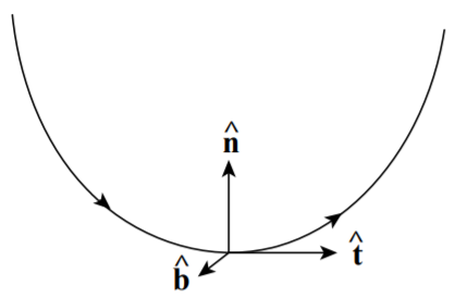
Frenet-Serret coordinates

The cartesian, polar, cylindrical, or spherical curvilinear coordinate systems, all are orthogonal coordinate systems that are fixed in space. There are situations where it is more convenient to use the Frenet-Serret coordinates which comprise an orthogonal coordinate system that is fixed to the particle that is moving along a continuous, differentiable, trajectory in three-dimensional Euclidean space. Let \(s(t)\) represent a monotonically increasing arc-length along the trajectory of the particle motion as a function of time \(t\). The Frenet-Serret coordinates, shown in Figure \(\PageIndex{4}\), are the three instantaneous orthogonal unit vectors \(\mathbf{\hat{t}}\), \(\mathbf{\hat{n}}\), and \(\mathbf{\hat{b}}\) where the tangent unit vector \(\mathbf{\hat{t}}\) is the instantaneous tangent to the curve, the normal unit vector \(\mathbf{\hat{n}}\) is in the plane of curvature of the trajectory pointing towards the center of the instantaneous radius of curvature and is perpendicular to the tangent unit vector \(\mathbf{\hat{t}}\), while the binormal unit vector is \(\mathbf{\hat{b}} =\mathbf{\hat{t}} \times \mathbf{\hat{n}}\) which is the perpendicular to the plane of curvature and is mutually perpendicular to the other two Frenet-Serrat unit vectors. The Frenet-Serret unit vectors are defined by the relations

\[\frac{d\mathbf{\hat{t}}}{ ds} = \kappa \mathbf{\hat{n}} \label{C.16}\]

\[\frac{d\mathbf{\hat{b}}}{ ds} = − \tau \mathbf{\hat{n}} \label{C.17}\]

\[\frac{d\mathbf{\hat{n}}}{ ds} = −\kappa \mathbf{\hat{t}}+ \tau \mathbf{\hat{b}} \label{C.18}\]

The curvature \(\kappa = \frac{1}{ \rho}\) where \(\rho\) is the radius of curvature and \(\tau\) is the torsion that can be either positive or negative. For increasing \(s\), a non-zero curvature \(\kappa\) implies that the triad of unit vectors rotate in a right-handed sense about \(\mathbf{\hat{b}}\). If the torsion \(\tau\) is positive (negative) the triad of unit vectors rotates in right (left) handed sense about \(\mathbf{\hat{t}}\).

Table \(\PageIndex{5}\): The differential relations plus a diagram of the corresponding unit vectors for the Frenet-Serret coordinate system.

Distance element	\(d\mathbf{s}(t) = \mathbf{\hat{t}} \left| \frac{d\mathbf{r}(t)}{dt} \right| dt = \mathbf{\hat{t}} v(t) dt\)
Unit vectors	\(\mathbf{\hat{t}}(t) = \frac{\mathbf{v}(t)}{ \left| v(t) \right|}\) \(\mathbf{\hat{n}}(t) = \frac{d\mathbf{\hat{t}}/dt}{\left| \mathbf{d\hat{t}}/dt \right|}\) \(\mathbf{\hat{b}} (t) = \mathbf{\hat{t}} \times \mathbf{\hat{n}}\)
Time derivatives of unit vectors	\(\frac{d}{d t} \begin{pmatrix} \mathbf{\hat{t}} \\ \mathbf{\hat{n}} \\ \mathbf{\hat{b}} \end{pmatrix} =|v|\begin{pmatrix} 0 & \kappa & 0 \\ -\kappa & 0 & \tau \\ 0 & -\tau & 0 \end{pmatrix} \begin{pmatrix} \mathbf{\hat{t}} \\ \mathbf{\hat{n}} \\ \mathbf{\hat{b}} \end{pmatrix}\)
Velocity	\(\mathbf{v} (t) = \frac{d\mathbf{r}(t)}{dt}\)
Acceleration	\(\mathbf{a}(t) = \frac{dv}{dt} \mathbf{\hat{t}} + \kappa v^2 \mathbf{\hat{n}}\)

Figure \(\PageIndex{4}\): Diagram for Table \(\PageIndex{5}\).

The above equations also can be rewritten in the form using a new unit rotation vector \(\boldsymbol{\omega}\) where

\[\boldsymbol{\omega}= \tau \mathbf{\hat{t}}+\kappa \mathbf{\hat{b}} \label{C.19}\]

Then equations \ref{C.16}−\ref{C.18} are transformed to

\[\frac{d\mathbf{\hat{t}}}{ ds} = \boldsymbol{\omega} \times \mathbf{\hat{t}} \label{C.20}\]

\[\frac{d\mathbf{\hat{n}}}{ ds} = \boldsymbol{\omega} \times \mathbf{\hat{n}} \label{C.21}\]

\[\frac{d\mathbf{\hat{b}}}{ ds} = \boldsymbol{\omega} \times \mathbf{\hat{b}} \label{C.22}\]

In general the Frenet-Serret unit vectors are time dependent. If the curvature \(\kappa = 0\) then the curve is a straight line and \(\mathbf{\hat{n}}\) and \(\mathbf{\hat{b}}\) are not well defined. If the torsion is zero then the trajectory lies in a plane. Note that a helix has constant curvature and constant torsion.

The rate of change of a general vector field \(\mathbf{E}\) along the trajectory can be written as

\[\frac{d\mathbf{E}}{ds} = \left( \frac{dE_t}{ ds} \mathbf{\hat{t}} + \frac{dE_n }{ds} \mathbf{\hat{n}}+ \frac{dE_b }{ds} \mathbf{\hat{b}} \right) + \boldsymbol{\omega} \times \mathbf{E} \label{C.23}\]

The Frenet-Serret coordinates are used in the life sciences to describe the motion of a moving organism in a viscous medium. The Frenet-Serret coordinates also have applications to General Relativity.

Problems

1. The goal of this problem is to help you understand the origin of the equations that relate two different coordinate systems. Refer to diagrams for cylindrical and spherical coordinates as your teaching assistant explains how to arrive at expressions for \(x_1\), \(x_2\), and \(x_3\) in terms of \(\rho \), \(\phi \), and \(z\) and how to derive expressions for the velocity and acceleration vectors in cylindrical coordinates. Now try to relate spherical and rectangular coordinate systems. Your group should derive expressions relating the coordinates of the two systems, expressions relating the unit vectors and their time derivatives of the two systems, and finally, expressions for the velocity and acceleration in spherical coordinates.