
23.8: Electric Generators


- Last updated
- Feb 20, 2022
- Save as PDF

( \newcommand{\kernel}{\mathrm{null}\,}\)
Learning Objectives
By the end of this section, you will be able to:
- Calculate the emf induced in a generator.
- Calculate the peak emf which can be induced in a particular generator system.
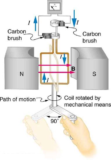
Electric generators induce an emf by rotating a coil in a magnetic field, as briefly discussed in "Induced Emf and Magnetic Flux." We will now explore generators in more detail. Consider the following example.
Example 23.8.1: Calculating the Emf Induced in a Generator Coil
The generator coil shown in Figure 23.8.1 is rotated through one-fourth of a revolution (from θ=0∘ to θ=90∘ ) in 15.0 ms. The 200-turn circular coil has a 5.00 cm radius and is in a uniform 1.25 T magnetic field. What is the average emf induced?
Strategy:
We use Faraday’s law of induction to find the average emf induced over a time Δt: emf=−NΔΦΔt. We know that N=200 and Δt=15.0ms, and so we must determine the change in flux ΔΦ to find emf.
Solution:
Since the area of the loop and the magnetic field strength are constant, we see that ΔΦ=Δ(BAcosθ)=ABΔ(cosθ). Now, Δ(cosθ)=−1.0, since it was given that θ goes from 0∘ to 90∘. Thus ΔΦ=−AB, and emf=NABΔt. The area of the loop is A=πr2=(3.14...)(0.0500m)2=7.85×10⁻³m2. Entering this value gives emf=200(7.85×10⁻³m2)(1.25T)1.50×10⁻³s=131V.
Discussion:
This is a practical average value, similar to the 120 V used in household power.
The emf calculated in the example is the average over one-fourth of a revolution. What is the emf at any given instant? It varies with the angle between the magnetic field and a perpendicular to the coil. We can get an expression for emf as a function of time by considering the motional emf on a rotating rectangular coil of width \w and height l in a uniform magnetic field, as illustrated in Figure 23.8.2.
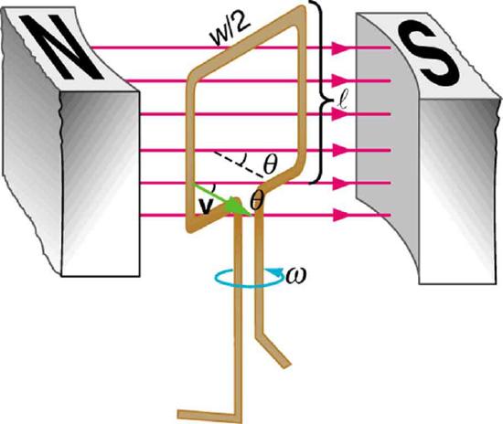
Charges in the wires of the loop experience the magnetic force, because they are moving in a magnetic field. Charges in the vertical wires experience forces parallel to the wire, causing currents. But those in the top and bottom segments feel a force perpendicular to the wire, which does not cause a current. We can thus find the induced emf by considering only the side wires. Motional emf is given to be emf=Blv, where the velocity v is perpendicular to the magnetic field B. Here the velocity is at an angle θ with B, so that its component perpendicular to B is vsinθ (Figure 23.8.2). Thus in this case the emf induced on each side is emf=Blvsinθ, and they are in the same direction. The total emf around the loop is then
emf=2Blvsinθ.
This expression is valid, but it does not give emf as a function of time. To find the time dependence of emf, we assume the coil rotates at a constant angular velocity ω. The angle θ is related to angular velocity by θ=ωt, so that
emf=2Blvsinωt.
Now, linear velovity v is related to angular velocity ω by v=rω. Here r=ω/2, so that v=(w/2)ω, and
emf=2Blw2ωsinωt=(w)Bωsinωt.
Noting that the area of the loop is A=w, and allowing for N loops, we find that
emf=NABωsinωt
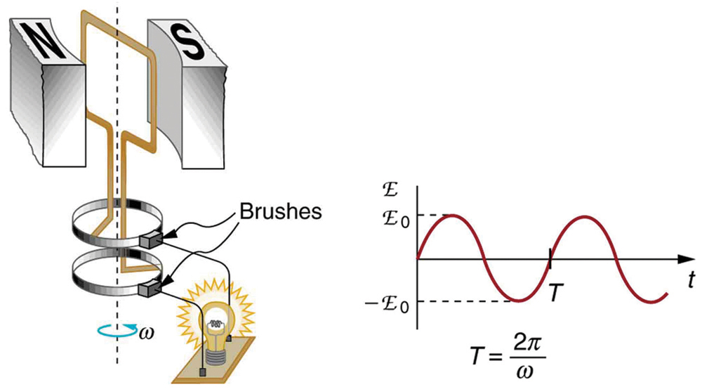
is the emf induced in a generator coil of N turns and area A rotating at a constant angular velocity ω in a uniform magnetic field B. This can also be expressed as
emf=emf0sinωt,
where emf0=NABω is the maximum (peak) emf. Note that the frequency of the oscillation is f=ω/2π, and the period is T=1/f=2π/ω. Figure 23.8.3 shows a graph of emf as a function of time, and it now seems reasonable that AC voltage is sinusoidal.
The fact that the peak emf, emf0=NABω, makes good sense. The greater the number of coils, the larger their area, and the stronger the field, the greater the output voltage. It is interesting that the faster the generator is spun (greater ω), the greater the emf. This is noticeable on bicycle generators—at least the cheaper varieties. One of the authors as a juvenile found it amusing to ride his bicycle fast enough to burn out his lights, until he had to ride home lightless one dark night.
Figure shows a scheme by which a generator can be made to produce pulsed DC. More elaborate arrangements of multiple coils and split rings can produce smoother DC, although electronic rather than mechanical means are usually used to make ripple-free DC.
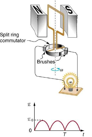
Figure 23.8.4: Split rings, called commutators, produce a pulsed DC emf output in this configuration.
Example 23.8.2: Calculating the Maximum Emf of a Generator
Calculate the maximum emf, emf0, of the generator that was the subject of Example.
Strategy
Once ω, the angular velocity, is determined, emf0=NABω can be used to find emf0. All other quantities are known.
Solution
Angular velocity is defined to be the change in angle per unit time:
ω=ΔθΔt.
One-fourth of a revolution is π/2 radians, and the time is 0.0150 s; thus,
ω=π/2rad0.0150s=104.7rad/s.
104.7 rad/s is exactly 1000 rpm. We substitute this value for ω and the information from the previous example into emf0=NABω, yielding
emf0=NABω=200(7.85×10⁻³m2)(1.25T)(104.7rad/s)=206V.
Discussion
The maximum emf is greater than the average emf of 131 V found in the previous example, as it should be.
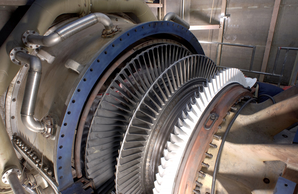
In real life, electric generators look a lot different than the figures in this section, but the principles are the same. The source of mechanical energy that turns the coil can be falling water (hydropower), steam produced by the burning of fossil fuels, or the kinetic energy of wind. 23.8.5 shows a cutaway view of a steam turbine; steam moves over the blades connected to the shaft, which rotates the coil within the generator.
Generators illustrated in this section look very much like the motors illustrated previously. This is not coincidental. In fact, a motor becomes a generator when its shaft rotates. Certain early automobiles used their starter motor as a generator. In Back Emf, we shall further explore the action of a motor as a generator.
Summary
- An electric generator rotates a coil in a magnetic field, inducing an emfgiven as a function of time by
emf=NABωsinωt,
where A is the area of an N-turn coil rotated at a constant angular velocity ω in a uniform magnetic field B.
- The peak emf \(emf_0) of a generator is
emf0=NABω.
Glossary
- electric generator
- a device for converting mechanical work into electric energy; it induces an emf by rotating a coil in a magnetic field
- emf induced in a generator coil
- emf=NABωsinωt, where A is the area of an N-turn coil rotated at a constant angular velocity ω in a uniform magnetic field B, over a period of time t
- peak emf
- (emf_0=NABω\)0=NABω