6.2: B-H Curves

The magnetic properties of ferromagnets at a fixed temperature are often described by curves of magnetic induction B vs. H, see Figure (6.2.3). H is the internal magnetic field: its sources include \(\rho_{m}=-\operatorname{div}(\vec{\text{M}})\) in the magnetic body as well as any externally applied magnetic field generated by a system of coils outside the magnetic body. \(\vec{\text{B}}=\mu_{0}(\vec{\text{H}}+\vec{\text{M}})\), and in the simplest case the three vectors \(\vec B\), \(\vec H\), \(\vec M\) are all parallel. Starting from the fully demagnetized state (H=0, M=0) the magnetization increases with H, and B follows the curve labeled ”virgin curve”. In the virgin state with H=0, an equal number of domains have positive magnetization as have negative magnetization so that the net magnetization is zero. As H increases those domains having a magnetization oriented along the applied field direction grow in volume at the expense of domains having a magnetization oriented opposite to the applied field direction. Eventually those domains having a component of magnetization opposed to the direction of H have been eliminated (at the point marked A in Figure (6.2.3)). However, iron has a cubic crystal structure and exhibits the property that the magnetization strongly prefers to orient itself along a direction corresponding to one of the three equivalent

Figure \(\PageIndex{3}\): A hysteresis loop for a polycrystalline specimen of pure iron. The details of the B-H loop are specimen sensitive. The saturation magnetization at room temperature is 2.14 Teslas. The remanent field is B_r= 1.22 T, and the coercive field is H_c= 79 Amps/m.

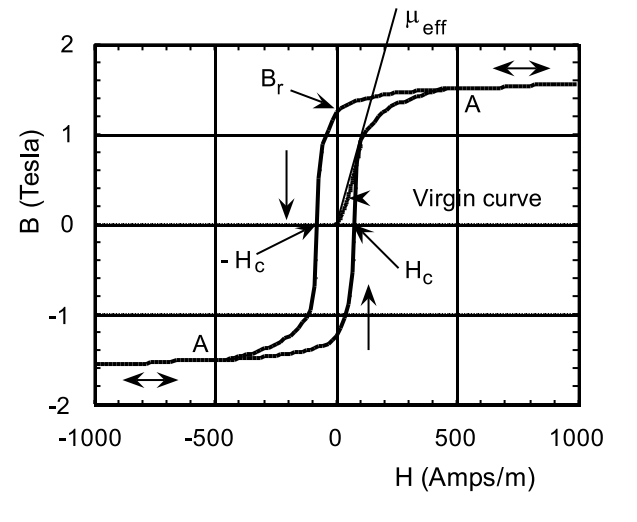
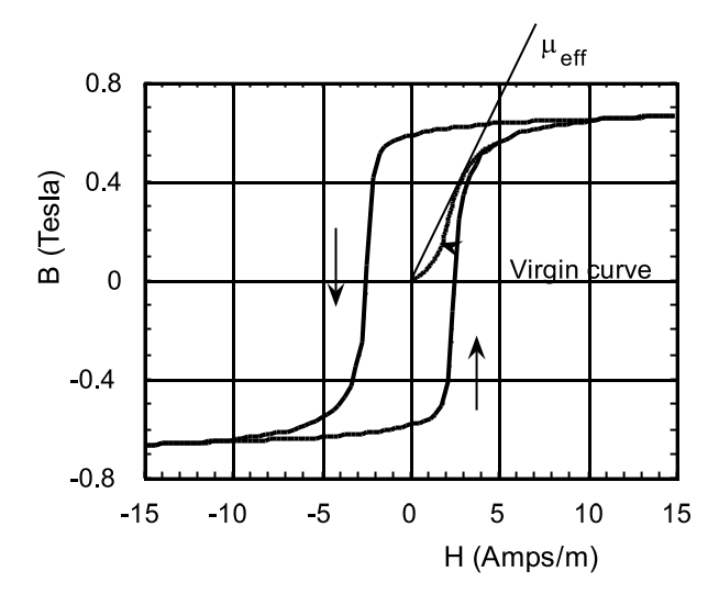
cubic axes. In a polycrystalline material at a field corresponding to point A in Figure (6.2.3) the domain magnetizations, each having a strength M_s per unit volume, are oriented at angles with respect to the applied field ranging from 0 to ±90^◦ . As H increases these domain magnetizations gradually rotate into the applied field direction: during this portion of the B-H loop the curve is reversible. Ultimately, the magnetization reaches the saturation value, M_s , and the magnetization density becomes uniform throughout the specimen. The field necessary to achieve the saturated state in iron, ∼ 2 × 10⁵ Amps/m, is very large because of the large magnetocrystalline anisotropy energy that resists the rotation of the magnetization away from a cubic axis. Very soft magnetic materials such as Supermalloy (79% Ni, 16% Fe, and 5% Mo, see Table (6.2.2)) have compositions corresponding to a relatively small magnetocrystalline anisotropy. The approach to saturation in such materials occurs at much lower applied fields than for iron, see Figure (6.2.4). It is also worth mentioning that a pure single crystal of iron for which the domain magnetizations are oriented along the cubic axes, Figure (6.1.2), exhibits a very large maximum effective permeability, see Table (6.2.2), and can be saturated in fields less than H= 100 Amps/m. However, polycrystalline iron is cheap and is therefore used extensively in the construction of electromagnets and large generators.

At saturation the magnetic domains have been eliminated so that the magnetization density is uniform throughout the body and has the value M_s . But \(\vec{\text{B}}=\mu_{0}(\vec{\text{H}}+\vec{\text{M}})\) so after saturation the B-field continues to increase with H, although the rate of increase of B with H becomes negligibly slow compared with the rate of increase leading up to saturation; the variation of B with H becomes imperceptible on the scale of Figure (6.2.3). Upon reducing the field H after having increased it to values larger than that corresponding to point A in Figure (6.2.3), B follows the upper curve in Figure (6.2.3) and when H=0 the magnetic induction reaches the remanent field value B = B_r . B gradually falls as domains with a reversed magnetization orientation gradually reform in the body. As H is further reduced B continues to follow the upper curve and eventually B reaches zero at a negative value of H called the coercive field, H_c. Continued reduction of H ultimately leads to magnetic saturation in the negative direction with uniform magnetization having the value -M_s . As H is increased from applied field values more negative than the field corresponding to point A in the third quadrant the B-field increases along the lower curve, the magnetization becomes less negative as the number of domains having

Figure \(\PageIndex{4}\): The hysteresis loop for the soft ferromagnet 4-79 Permalloy (79% Ni, 17% Fe, 4% Mo). The maximum effective permeability is 0.14 (the relative permeability is µ_R = 1.1×10⁵ ), and H_c = 2.45 Amps/m. The saturation field is B_s= 0.87 Teslas.

a positive magnetization increases, and ultimately B becomes positive. At the coercive field H_c the magnetic induction is zero; B=0. At sufficiently large values of the magnetic field the specimen once again becomes saturated with a uniform magnetization having the value Ms. For fields larger than 500 Amps/m, or for fields less than -500 Amps/m, the curve of B vs. H is reversible. The loop defined by the upper and lower curves in Figure (6.2.3) is called a major hysteresis loop. Two questions arise immediately: (1) What happens if H is decreased before point A is reached? and (2) How can the virgin state with H=0, M=0, and B=0 be attained? If H is reduced before the reversible part of the B-H loop has been attained the B-field decreases along a minor hysteresis loop such as those shown in Figure (6.2.5). If a sinusoidal driving field is applied having an amplitude sufficient to drive the specimen into the reversible part the hysteresis loop the magnetic state is carried around the hysteresis loop from one extreme in the plus direction to an extreme in the negative direction many times per second. If now the amplitude of the driving field is slowly reduced to zero the hysteresis curve collapses to zero symmetrically around the origin. The specimen will be left in the virgin state in which B=M=H=0.

Important parameters associated with the hysteresis loop are (1) the remanent field, B_r , (2) the coercive field, H_c, and (3) the maximum effective permeability defined by the maximum slope of the straight line joining the origin to a point on the virgin magnetization curve as shown in Figures (6.2.3, 6.2.4). There are two major classes of ferromagnetic materials: soft ferromagnets and hard ferromagnets. Soft magnetic materials are characterized by very small values of the coercive field, see Table (6.2.2). For such materials the dependence of B on H is almost linear for H < H_c, and as a reasonable approximation one can write \(\vec{\text{B}}=\mu_{e f f} \vec{\text{H}}\). It is useful to express the effective permeability as a dimensionless number

\[\mu_{e f f}=\mu_{R} \mu_{0} .\nonumber \]

Pure polycrystalline iron is a soft ferromagnet characterized by H_c = 60 Amps/m and µ_eff= 0.013, or µ_R ∼ 10,000. There are a number of alloys that behave very nearly like perfectly soft ferromagnets, see Table (6.2.2).

Hard magnetic materials are characterized by large values of the coercive field and remanent field B_r , see Table (6.2.3). Very hard ferromagnets such as SmCo alloys, NdFeB alloys, and Strontium ferrites can be better described in terms of M vs. H. The variation of magnetization with internal magnetic field, H, is shown for a commercial Barium ferrite in Figure (6.2.6); only negative

Figure (6.2.4). For the lowest minor loop the field was reduced after having partially traversed the virgin magnetization curve. For the upper minor loop the field was reduced after having traversed the major hysteresis curve cycle at least once.

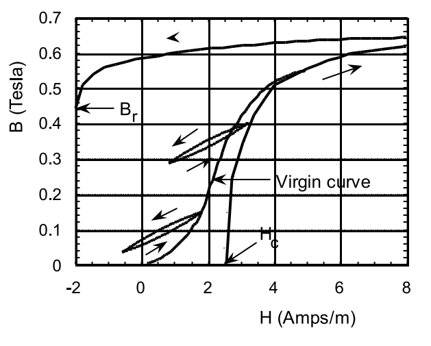
Table \(\PageIndex{2}\): Magnetic properties of some soft magnetic materials. B = µ_eff (H + M), where µ_eff = µ_Rµ₀. One Tesla equals 10 kGauss, and 79 Amps/m equals 1 Oersted. Permalloy is an alloy of 78.5 atomic % Ni and 21.5 atomic % Fe. Supermalloy is composed of 79 atomic % Ni, 16 atomic % Fe, and 5 atomic % Mo.

Figure \(\PageIndex{6}\): The variation with internal magnetic field, H, of the magnetization at room temperature for a commercial Strontium Ferrite. The coercive field is 2.59 × 10⁵ Amps/m.

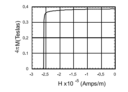
internal fields, H, are shown because this portion of the magnetization curve is the one required for practical applications. The hysteresis loop is very nearly rectangular, meaning that to a good approximation the magnetization is independent of the H-field until it flips 180^◦ at, or near, the coercive field. For very hard materials such as those listed in Table (6.2.3) the concept of a permeability is not very useful.

Warning! Commercial hysteresis loops are usually displayed using CGS units. In the CGS system the fields B,M,H all have the same units, although for historical reasons the units of B,M are called Gauss whereas the units of H are called Oersteds. The conversion from CGS to MKS units is relatively simple: 1 Tesla= 10,000 Gauss. 79.6 Amps/m = 1 Oersted. M in Amps/m = [4\(\pi\)M(in Gauss)] × 79.6.

In the CGS system \(\vec{\text{B}}=\vec{\text{H}}+4 \pi \vec{\text{M}}\). The relative permeability is the same ~ for both systems.

Table \(\PageIndex{3}\): Magnetic properties of some commercial hard magnet materials. (See, for example, www.dextermag.com).

Figure \(\PageIndex{7}\): Device for measuring the axial magnetic field, B, inside a cylinder having a cross-sectional area A. A coil of N turns is connected to a voltmeter V.

Figure \(\PageIndex{8}\): A plot of B inside a long iron rod vs the externally applied magnetic field H₀ = B₀/µ₀. The length to diameter ratio is 25 corresponding to a demagnetizing coefficient N_z= 0.00467.

6.2.1 Measuring the B-H Loop.

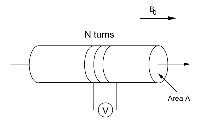
It is relatively easy to measure the axial magnetic flux density, B, in a specimen. It is only necessary to wind a few turns of wire closely around a specimen and to measure the emf developed across the coil terminals as an external field B₀ is changed with time, see Figure (6.2.7). The emf across the coil terminals is given by Faraday’s law:

\[\text{V}(\text{t})=\text{NA} \frac{\text{dB}}{\text{dt}} , \nonumber \]

where N is the number of turns on the coil and A is the cross-sectional area of the specimen in m² . Upon integration of the voltage signal starting from a known initial condition (B=0 at t=0 say) one obtains B inside the specimen corresponding to a particular value of the applied field H₀ = B₀/µ₀. In this way one can trace out the hysteresis loop of B vs H₀ as the specimen is saturated first in one direction and then in the other direction. Unfortunately the hysteresis loop so obtained is not what is wanted: it depends more on the geometry of the specimen than on its intrinsic magnetic properties.

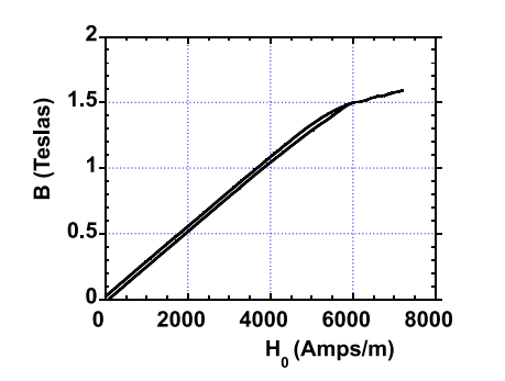
What is wanted is the variation of B inside the cylinder with the value of H inside the cylinder. But H inside the cylinder is the sum of the applied field H₀ = B₀/µ₀ plus the contribution generated by the magnetic pole density distribution \(\rho_{M}=-\operatorname{div}(\vec{\text{M}})\). This pole field very nearly cancels out the applied field H₀ in a material having a large permeability. The net result is that the curve of B vs H₀ measures an effective demagnetizing coefficient for the body under test, and does not provide a satisfactory measure of an intrinsic magnetic property of the material of the test body. In order to see how this comes about consider a particular example: consider a cylindrical bar whose length is 25 times its diameter (25 cm long by 1 cm in diameter, for example). Let this bar be characterized by the hysteresis loop shown in Figure (6.2.3). The pole field inside this bar can be approximated by H_D = −N_zM, where N_z is the demagnetizing factor for an ellipsoid of revolution having the same length to diameter ratio as the cylinder; M is the magnetization density in the bar. The demagnetization factor for an ellipsoid of revolution having a length to diameter ratio of 25 is N_z=0.00467; see Chpt.(2), Figure (2.7.19) and eqn.(2.5.1). Inside the rod one has B/µ₀ = H+M. Given the co-ordinates of a point on the B-H loop one can calculate the magnetization, M. Consider the point in Figure (6.2.3) B=1.0 Tesla and H=110 Amps/m. For this point B/µ₀ = 1.0/(4\(\pi\) × 10⁻⁷ ) = 0.796 × 10⁶ Amps/m. Thus H is negligible and M= 0.796 × 10⁶ Amps/m. The resulting pole field is H_D = −N_zM = −3.72 × 10³ Amps/m. In order to obtain a net value H= +110 Amps/m it is necessary to apply a field H₀ = (3.72×10³ )+110 Amps/m for a total field H₀ = 3.83×10³ Amps/m. In this same way one can calculate B vs H₀ for all of the points on the hysteresis loop. The results of such a calculation are shown in Figure (6.2.8). The most obvious result is that B is nearly a linear function of the applied field H₀ for H₀ less than 5800 Amps/m; the slope of the line corresponds to a relative permeability µ_R= 212 (NB. 1/N_z= 214). Moreover, the hysteretic behaviour has been reduced to a very small value: approximately 0.05 Tesla in B. It is easy to show that if the material properties are such that B= µ_Rµ₀H then for large µR one has B= µ₀H₀/N_z; ie. a straight line having a slope corresponding to µ_R = 1/N_z. The argument runs as follows:

\[\begin{aligned}
\text{B} &=\mu \text{H}=\mu_{0}(\text{H}+\text{M}), \\
& \frac{\mu}{\mu_{0}} \text{H}=(\text{H}+\text{M}),
\end{aligned} \nonumber \]

so

\[\text{M}=\left(\mu_{R}-1\right) \text{H} .\nonumber \]

Since the pole field is H_D = −N_zM, the applied field must overcome this pole field and in addition supply the field H. Therefore the applied field is given

Figure \(\PageIndex{9}\): A ring shaped specimen used to measure the intrinsic magnetic properties of a soft magnetic material. The primary winding of N_p turns is used to generate the field H. The secondary coil of N_s turns is used to measure the field B in the ring.

by

\[\text{H}_{0}=\text{N}_{\text{z}}\left(\mu_{R}-1\right) \text{H}+\text{H}, \nonumber \]

or

\[\text{H}=\frac{\text{H}_{0}}{\left[\text{N}_{\text{z}}\left(\mu_{R}-1\right)+1\right]} , \nonumber \]

and

\[\text{B}=\frac{\mu_{0} \mu_{R} \text{H}_{0}}{\left[\text{N}_{\text{z}}\left(\mu_{R}-1\right)+1\right]} . \nonumber \]

Upon dividing through by µ_R and taking the limit such that µ_R ≫ 1, one obtains

\[ \text{B} \cong \mu_{0} \text{H}_{0} / \text{N}_{\text{z}} . \label{6.3}\]

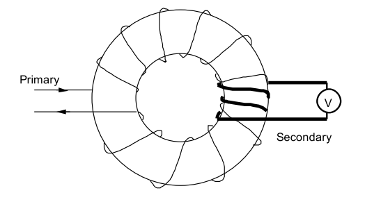
The point is that in order to measure the intrinsic response of a soft magnetic material it is necessary to avoid spatial variations in the magnetization that give rise to magnetic pole fields. This can be done by using a specimen having the topology of a ring, Figure (6.2.9). This ring can be supplied with a uniformly wound primary coil of N_p turns used to generate the applied field, H₀, plus a secondary coil of N_s turns used to measure the flux density in the specimen. There are no magnetic poles if M is uniform around the ring, therefore the field in the material is just H = N_pI/L, where I is the primary coil current in Amps and L is the length in meters measured along the centerline of the ring. The B-field can be calculated from the emf developed across the secondary windings as the primary current is changed; according to Faraday’s law

\[\text{V}=\text{N}_{\text{s}} \text{A}(\text{dB} / \text{dt}) , \nonumber \]

where A is the cross-sectional area of the ring.