9.1: Introduction to Plane Waves

An electric dipole directed along z, located at the origin, and oscillating with the circular frequency $ω$ produces electric and magnetic fields far from the origin that have the form (see equations (7.4.5)):

$$\begin{align} \mathrm{E}_{\theta} &=-\frac{\omega^{2}}{4 \pi \epsilon_{0}} \frac{\mathrm{p}_{0} \sin \theta}{\mathrm{c}^{2} \mathrm{R}} \exp (-i \omega[\mathrm{t}-\mathrm{R} / \mathrm{c}]), \label{9.1} \\ \mathrm{B}_{\phi} &=\mathrm{cE}_{\theta} \nonumber \\ \mathrm{H}_{\phi} &=-\frac{\omega^{2}}{4 \pi} \frac{\mathrm{p}_{0} \sin \theta}{\mathrm{cR}} \exp (-i \omega[\mathrm{t}-\mathrm{R} / \mathrm{c}]) \nonumber \end{align}$$

where $\text{p}_{\text{z}}=\text{p}_{0} \exp (-i \omega[\text{t}-\text{R} / \text{c}])$, and t is the time at which the observer at $\vec R$ measures the fields. It must always be kept in mind that the fields are represented by real numbers; the notation of complex numbers is simply a convenient book-keeping device for dealing with sinusoidal functions. The notation $\exp (-i \omega\text{t})$ “the real part of $\exp (-i \omega\text{t})$” i.e. $\cos (\omega\text{t})$. It is particularly important to remember this when calculating the Poynting vector or the energy densities which involve the product of two field amplitudes. For example, the Poynting vector corresponding to the fields of Equations ($\ref{9.1}$) is given by

$$\text{S}_{\text{r}}=\text{E}_{\theta} \text{H}_{\phi}=\frac{1}{4 \pi \epsilon_{0}} \frac{\omega^{4}}{4 \pi} \frac{\text{p}_{0}^{2} \sin ^{2} \theta}{\text{c}^{3} \text{R}^{2}} \cos ^{2}(\omega[\text{t}-\text{R} / \text{c}]) \label{9.2}$$

Note that the time factor is not the same as

$$\text {Real }(\exp (-2 i \omega[\text{t}-\text{R} / \text{c}]))=\cos (2 \omega[\text{t}-\text{R} / \text{c}]). \label{9.3}$$

The time average of Equation ($\ref{9.3}$) is zero, whereas the time average of the correct expression, Equation ($\ref{9.2}$), is given by

$$<\text{S}_{\text{r}}>=\left(\frac{1}{8 \pi}\right)\left(\frac{\text{c}}{4 \pi \epsilon_{0}}\right)\left(\frac{\omega}{\text{c}}\right)^{4} \frac{\text{p}_{0}^{2} \sin ^{2} \theta}{\text{R}^{2}}, \label{9.4}$$

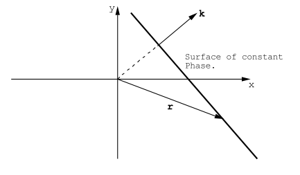
since the time average of the cosine squared function is 1/2. At distances far removed from the dipole radiator the surface of constant R can be approximated locally by a plane perpendicular to $\hat{\text{u}}_{\text{r}}$, a unit vector parallel with $\vec R.$ This suggests that Maxwell’s equations ought to have plane wave solutions of the form

$$\vec{\text{E}}(\vec{\text{r}}, \text{t})=\vec{\text{E}}_{0} \exp (i[\vec{\text{k}} \cdot \vec{\text{r}}-\omega \text{t}]), \label{9.5}$$

$$\vec{\text{B}}(\vec{\text{r}}, \text{t})=\vec{\text{B}}_{0} \exp (i[\vec{\text{k}} \cdot \vec{\text{r}}-\omega \text{t}]),\nonumber$$

where $\vec k$ is a vector whose magnitude is $\omega / c$ and whose direction lies along the direction of propagation of the wave, and where $\vec{\text{E}}_{0}$ and $\vec{\text{B}}_{0}$ are constant vectors that are perpendicular to each other and to the wave-vector $\vec k$ (see Figure (9.1.1)).

Equations ($\ref{9.5}$) can be written in component form using some convenient co-ordinate system, and using $\operatorname{Real}(\exp (i[\vec{\text{k}} \cdot \vec{\text{r}}-\omega \text{t}]))=\cos (\vec{\text{k}} \cdot \vec{\text{r}}-\omega \text{t})$:

$$\begin{array}{l} \text{E}_{\text{x}}=\text{E}_{0 x} \cos \left(\text{k}_{\text{x}} \text{x}+\text{k}_{\text{y}} \text{y}+\text{k}_{\text{z}} \text{z}-\omega \text{t}\right), \\ \text{E}_{\text{y}}=\text{E}_{0 y} \cos \left(\text{k}_{\text{x}} \text{x}+\text{k}_{y} \text{y}+\text{k}_{\text{z}} \text{z}-\omega \text{t}\right), \\ \text{E}_{\text{z}}=\text{E}_{0 z} \cos \left(\text{k}_{\text{x}} \text{x}+\text{k}_{y} \text{y}+\text{k}_{\text{z}} \text{z}-\omega \text{t}\right), \\ \text{B}_{\text{x}}=\text{B}_{0 x} \cos \left(\text{k}_{\text{x}} \text{x}+\text{k}_{\text{y}} \text{y}+\text{k}_{\text{z}} \text{z}-\omega \text{t}\right), \\ \text{B}_{\text{y}}=\text{B}_{0 y} \cos \left(\text{k}_{\text{x}} \text{x}+\text{k}_{\text{y}} \text{y}+\text{k}_{\text{z}} \text{z}-\omega \text{t}\right), \\ \text{B}_{\text{z}}=\text{B}_{0 z} \cos \left(\text{k}_{\text{x}} \text{x}+\text{k}_{y} \text{y}+\text{k}_{\text{z}} \text{z}-\omega \text{t}\right), \end{array} \label{9.6}$$

Using these expressions it is easy to show that

$$\operatorname{curl}(\vec{\text{E}})=-\left(\vec{\text{k}} \times \vec{\text{E}}_{0}\right) \sin (\vec{\text{k}} \cdot \vec{\text{r}}-\omega \text{t}), \nonumber$$

Figure $\PageIndex{1}$: A plane wave propagating along the direction specified by $\vec k$ and for which $|\vec{\text{k}}|=\text{k}=\omega / \text{c}$. For an electromagnetic plane wave in free space for which the fields $\vec E$ and $\vec B$ satisfy Maxwell’s equations, both $\vec E$ and $\vec B$ lie in the surface of constant phase and are perpendicular to each other.

$$\begin{aligned} \operatorname{div}(\vec{\text{E}}) &=-\left(\vec{\text{k}} \cdot \vec{\text{E}}_{0}\right) \sin (\vec{\text{k}} \cdot \vec{\text{r}}-\omega \text{t}), \\ \operatorname{curl}(\vec{\text{B}}) &=-\left(\vec{\text{k}} \times \vec{\text{B}}_{0}\right) \sin (\vec{\text{k}} \cdot \vec{\text{r}}-\omega \text{t}), \\ \operatorname{div}(\vec{\text{B}}) &=-\left(\vec{\text{k}} \cdot \vec{\text{B}}_{0}\right) \sin (\vec{\text{k}} \cdot \vec{\text{r}}-\omega \text{t}), \end{aligned} \nonumber$$

In free space Maxwell’s equations become

$$\begin{align} \operatorname{curl}(\overrightarrow{\mathrm{E}}) &=-\frac{\partial \overrightarrow{\mathrm{B}}}{\partial \mathrm{t}}, \label{9.7} \\ \operatorname{curl}(\overrightarrow{\mathrm{B}}) &=\epsilon_{0} \mu_{0} \frac{\partial \overrightarrow{\mathrm{E}}}{\partial \mathrm{t}}, \nonumber \\ \operatorname{div}(\overrightarrow{\mathrm{E}}) &=0, \nonumber \\ \operatorname{div}(\overrightarrow{\mathrm{B}}) &=0. \nonumber \end{align}$$

Figure $\PageIndex{2}$: An electromagnetic plane wave propagating in free space. The electric field vector,$\vec{\text{E}}(\vec{\text{r}}, \text{t})=\vec{\text{E}}_{0} \cos (\vec{\text{k}} \cdot \vec{\text{r}}-\omega \text{t})$, and the magnetic field vector, $\vec{\text{B}}(\vec{r}, t)=\vec{\text{B}}_{0} \cos (\vec{\text{k}} \cdot \vec{r}-\omega t)$, along with the propagation vector, $\vec k$, form a right handed orthogonal triad.

Substitution of Equations ($\ref{9.6}$) into Maxwell’s Equations ($\ref{9.7}$) gives

$$\vec{\text{k}} \times \vec{\text{E}}_{0}=\omega \vec{\text{B}}_{0},$$

$$\vec{\text{k}} \times \vec{\text{B}}_{0}=-\epsilon_{0} \mu_{0} \omega \vec{\text{E}}_{0},\nonumber$$

$$\vec{\text{k}} \cdot \vec{\text{E}}_{0}=0,\nonumber$$

$$\vec{\text{k}} \cdot \vec{\text{B}}_{0}=0.\nonumber$$

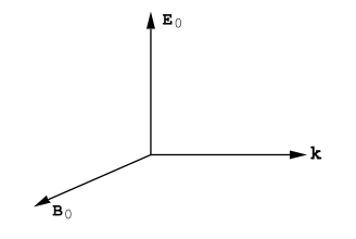
The last two equations state that for plane wave solutions of Maxwell’s equations in free space both the electric and magnetic field vectors must be perpendicular to the direction of propagation specified by the vector $\vec k$; i.e. $\vec{\text{E}}_{0}$ and $\vec{\text{B}}_{0}$ must be parallel with the surfaces of constant phase. The first two equations of (9.1.8) state that the fields $\vec{\text{E}}_{0}$ and $\vec{\text{B}}_{0}$ must be mutually perpendicular; thus the three vectors $\vec{\text{E}}_{0}$, $\vec{\text{B}}_{0}$, and $\vec k$ form an orthogonal right handed triad. In order to satisfy Maxwell’s equations the magnitude of the wave-vector must be given by

$$\text{k}^{2}=\epsilon_{0} \mu_{0} \omega^{2}=\left(\frac{\omega}{\text{c}}\right)^{2},\label{9.9}$$

and the amplitudes of the electric and magnetic fields must be related by

$$\left|\vec{\text{E}}_{0}\right|=\text{c}\left|\vec{\text{B}}_{0}\right| , \nonumber$$

see Figure (9.1.2). Notice that E and B oscillate in phase: ie. they have exactly the same sinusoidal dependence on space and on time. These relations are the same as those which were earlier associated with the wave produced by an oscillating dipole, Equations (7.4.5).

In free space the displacement vector, $\vec D$, is related to the electric field by $\vec{\text{D}}=\epsilon_{0} \vec{\text{E}}$ so that the time rate of change of the energy density stored in the electric field, Equation (8.2.6), becomes

$$\frac{\partial \text{W}_{\text{E}}}{\partial \text{t}}=\epsilon_{0} \vec{\text{E}} \cdot \frac{\partial \vec{\text{E}}}{\partial \text{t}}=\frac{\partial}{\partial \text{t}}\left(\frac{\epsilon_{0} \text{E}^{2}}{2}\right) .\label{9.10}$$

Using (9.1.10), the energy density stored in the electric field of a plane wave is given by

$$\text{W}_{\text{E}}=\frac{\epsilon_{0} \text{E}_{0}^{2}}{2} \cos ^{2}(\vec{\text{k}} \cdot \vec{\text{r}}-\omega \text{t}), \quad \text { Joules} / \text{m}^{3},\nonumber$$

This energy density oscillates in both space and time, in particular at a fixed point in space the energy density periodically vanishes. However, the average energy density measured at any point in space is independent of both position and time:

$$<\text{W}_{\text{E}}>=\frac{\epsilon_{0}}{4} \text{E}_{0}^{2}, \quad \text { Joules} / \text{m}^{3}, \label{9.11}$$

Similarly, the time rate of change of the energy density stored in the magnetic field is given by (8.7)

$$\frac{\partial \text{W}_{\text{B}}}{\partial \text{t}}=\vec{\text{H}} \cdot \frac{\partial \vec{\text{B}}}{\partial \text{t}}=\frac{\partial}{\partial \text{t}}\left(\frac{\text{B}^{2}}{2 \mu_{0}}\right). \label{9.12}$$

Therefore one can write

$$\text{W}_{\text{B}}=\frac{\text{B}^{2}}{2 \mu_{0}}=\frac{\text{B}_{0}^{2}}{2 \mu_{0}} \cos ^{2}(\vec{\text{k}} \cdot \vec{\text{r}}-\omega \text{t}) \quad \text { Joules} / m^{3}.\nonumber$$

The time averaged energy density stored in the magnetic field is independent of position and since $\text{B}=\text{E} / \text{c}$ is given by

$$<\text{W}_{\text{B}}>=\frac{\text{B}_{0}^{2}}{4 \mu_{0}}=\frac{\text{E}_{0}^{2}}{4 \mu_{0} \text{c}^{2}}=\frac{\epsilon_{0} \text{E}_{0}^{2}}{4}=<\text{W}_{\text{E}}>\quad \text { Joules} / m^{3}. \label{9.13}$$

The average energy density stored in the magnetic field is exactly the same, in free space, as the average energy density stored in the electric field. The total time averaged energy density stored in the electromagnetic field is

$$<\text{W}>=<\text{W}_{\text{E}}>+<\text{W}_{\text{B}}>=\frac{\epsilon_{0} \text{E}_{0}^{2}}{2}, \quad \text { Joules} / m^{3}. \label{9.14}$$

The average rate at which energy in the electromagnetic field is transported across a unit area normal to the direction of propagation, i.e. normal to $\vec k$, can be obtained by multiplying Equation ($\ref{9.14}$) by the speed of light: this rate is also just the time average of the Poynting vector

$$<\text{S}>=\text{c} \frac{\epsilon_{0} \text{E}_{0}^{2}}{2}=\frac{1}{2} \sqrt{\frac{\epsilon_{0}}{\mu_{0}}} \text{E}_{0}^{2}, \quad \text { Watts } / \text{m}^{2}. \label{9.15}$$

The quantity $\text{Z}_{0}=\sqrt{\mu_{0} / \epsilon_{0}}$ has the units of a resistance; it is called the impedance of free space, and $\text{Z}_{0}=377$ Ohms. From the equations for the space and time variation of a plane wave, Equations ($\ref{9.6}$), it follows that for a fixed time the electric and magnetic fields vary in space with a period along the direction of $vec k$ given by $2 \pi /|\vec{k}|.$ By definition, this spatial period is the wavelength, λ, therefore $|\vec{\text{k}}|=2 \pi / \lambda.$ Similarly, at a fixed position in space the fields oscillate in time with the period $2 \pi / \omega;$ by definition, this period, T, is the inverse of the frequency,f, therefore $\omega=2 \pi \text{f}$. In order to satisfy Maxwell’s equations, the frequency and wavelength of a plane wave are related by Equation ($\ref{9.9}$)

$$\omega=\text{c}|\vec{\text{k}}|;\nonumber$$

this can be written in the more familiar form $\text{f} \lambda=\text{c}.$