9.4: Gaussian Light Beams

It is impossible to generate an unbounded plane wave, of course. Nevertheless, the concept of unbounded plane waves is a very useful one because a finite beam of radiation can be described as the superposition of plane waves having different amplitudes and phases and propagating in slightly different directions, see Figure (9.3.8). To simplify matters let us assume that the amplitude function, A(p,q), is symmetric in p,q: ie. A(-p,-q)= A(p,q). This simplification allows one to construct a beam in which the electric field is polarized along a particular direction in the plane- along the x-direction, say. Eqn.(\ref{9.21}) illustrates how such a beam could be constructed:

\[\text{E}_{\text{x}}(\text{x}, \text{y}, \text{z}, \text{t})=\int \int_{-\infty}^{\infty} \operatorname{dpdq} \text{A}(\text{p}, \text{q}) \exp (i[\text{px}+\text{qy}+\text{kz}-\omega \text{t}]), \label{9.21}\]

where

\[\text{p}^{2}+\text{q}^{2}+\text{k}^{2}=\left(\frac{\omega}{\text{c}}\right)^{2}=\text{k}_{0}^{2}, \nonumber \]

Eqn.(\ref{9.21}) is an example of a Fourier Integral. The amplitude function A(p,q) can be chosen to give the required beam profile in the x-y plane at some plane z=constant; it is convenient to choose this plane to be at z=0. The beam profile at any other position z can be obtained using the integral (\ref{9.21}). As an example of how this works let us treat a specific case for which the mathematics can be easily worked out. Suppose that at z=0 the beam cross-section can be described as a plane wave whose amplitude falls off exponentially along x and y:

\[\text{E}_{\text{x}}(\text{x}, \text{y}, 0)=\text{E}_{0} \exp \left(\frac{-\left(\text{x}^{2}+\text{y}^{2}\right)}{\text{w}_{0}^{2}}\right). \label{9.22}\]

A time dependence exp (−iωt) is assumed, but this factor will be suppressed in the following. The output beam from a typical gas laser, a He-Ne laser for example, exhibits the spatial variation (\ref{9.22}) at the output mirror with w₀ approximately equal to 1 mm. Such a beam profile is called a Gaussian beam profile. The spatial Fourier integral in (\ref{9.21}) can be inverted for z=0 to obtain

\[\text{A}(\text{p}, \text{q})=\frac{1}{4 \pi^{2}} \int \int_{-\infty}^{\infty} \operatorname{dxdy} \text{E}_{\text{x}}(\text{x}, \text{y}, 0) \exp (-i[\text{px}+\text{qy}]). \label{9.23}\]

Using the Gaussian spatial variation of Equation (\ref{9.22}) one finds

\[\text{A}(\text{p}, \text{q})=\frac{\text{E}_{0} \text{w}_{0}^{2}}{4 \pi} \exp \left(-\frac{\text{w}_{0}^{2}}{4}\left(\text{p}^{2}+\text{q}^{2}\right)\right). \label{9.24}\]

The Fourier transform of a Gaussian function is another Gaussian function: see section(9.4.1).

Notice that the amplitude function (\ref{9.24}) becomes very small if p² or q² is greater than \(4 / \text{w}_{0}^{2}\): : this means that the waves in the bundle describing the radiation beam that have transverse components p,q much larger than ±2/w₀ can be neglected. In a typical case the laser beam radius is ∼1 mm so that the amplitude A(p,q) becomes small for | p |, | q | larger than 2 × 10³ m⁻¹ . But at optical frequencies λ ∼ (1/2)×10⁻⁶ m so that k₀ ∼ 2\(\pi\)/λ ∼ 4\(\pi\) ×10⁶ m⁻¹ . Thus the important values of the transverse components p,q of the plane waves that make up the beam are very small compared with the total wavevector k₀. The longitudinal component of the wave-vector, the z-component k, is given by

\[\text{k}^{2}=\left(\frac{\omega}{\text{c}}\right)^{2}-\text{p}^{2}-\text{q}^{2}=\text{k}_{0}^{2}-\text{p}^{2}-\text{q}^{2}. \nonumber \]

Figure \(\PageIndex{9}\): The variation of the phase across the x-y plane for a spherical wave is described by exp \(\left(\frac{i k_{0}}{2 R}\left(x^{2}+y^{2}\right)\right)\). The phase increases with distance, r, in the plane because the distance from the center of curvature to an off-axis point on the plane is larger than the radius of curvature R.

But \(\left(p^{2}+q^{2}\right) / k_{0}^{2}\) is much less than unity so that one can write

\[\text{k} \approx \text{k}_{0}-\frac{\left(\text{p}^{2}+\text{q}^{2}\right)}{2 \text{k}_{0}}. \label{9.25}\]

Now using the approximation Equation (\ref{9.25}) in Equation (\ref{9.21}) investigate the beam profile at some arbitrary value of z:

\[\begin{align}
\mathrm{E}_{\mathrm{x}}(\mathrm{x}, \mathrm{y}, \mathrm{z})=& \frac{\mathrm{E}_{0} \mathrm{w}_{0}^{2}}{4 \pi} \int \int_{-\infty}^{\infty} \operatorname{dpdq} \exp \left(-\frac{\mathrm{w}_{0}^{2}}{4}\left[\mathrm{p}^{2}+\mathrm{q}^{2}\right]\right). \label{9.26} \\
& \cdot \exp (i[\mathrm{px}+\mathrm{qy}]) \exp \left(-i \frac{\left[\mathrm{p}^{2}+\mathrm{q}^{2}\right] \mathrm{z}}{2 \mathrm{k}_{0}}\right) \exp \left(i \mathrm{k}_{0} \mathrm{z}\right) \nonumber
\end{align}\]

The integrals in Equation (\ref{9.26}) can be evaluated to obtain

\[\text{E}_{\text{x}}(\text{x}, \text{y}, \text{z})=\frac{\text{E}_{0}}{\sqrt{1+\left(\text{z} / \text{z}_{\text{R}}\right)^{2}}} \exp \left(\frac{i \text{k}_{0}}{2 \tilde{\text{q}}}\left(\text{x}^{2}+\text{y}^{2}\right)\right) \exp \left(i\left[\text{k}_{0} \text{z}-\psi\right]\right), \label{9.27}\]

where

\[\tilde{\text{q}}=\text{z}-\text{i} \text{z}_{\text{R}}, \label{9.28}\]

\[\text{z}_{\text{R}}=\frac{\text{k}_{0} \text{w}_{0}^{2}}{2}=\frac{\pi \text{w}_{0}^{2}}{\lambda}, \label{9.29}\]

and

\[\tan (\psi)=\text{z} / \text{z}_{\text{R}}. \label{9.30}\]

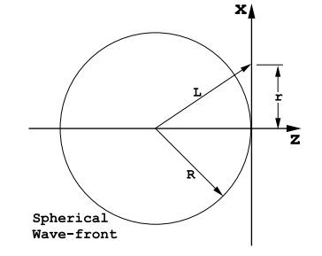
See Section(9.4.2) for the details of the calculation. The variable \(\tilde{\text{q}}\) is called the complex radius of curvature of the beam. This nomenclature stems from the description of a spherical wave-front, Figure (9.4.9) as will be explained in the next paragraph. The length z_R is called the Rayleigh range.

A spherical wave-front exhibits a phase variation across a plane perpendicular to the direction of propagation given by

\[\exp \left(\frac{i \text{k}_{0}}{2 \text{R}}\left(\text{x}^{2}+\text{y}^{2}\right)\right), \nonumber \]

where R is the radius of curvature. A comparison of this expression with Equation (\ref{9.27}) shows why \(\tilde{\text{q}}\) is called the complex radius of curvature. One can separate the reciprocal of the complex radius of curvature into its real and imaginary parts:

\[\frac{1}{\tilde{\text{q}}}=\frac{1}{\text{z}-\text{z}_{\text{R}}}=\frac{\text{z}+\text{i} \text{z}_{\text{R}}}{\text{z}^{2}+\text{z}_{\text{R}}^{2}}. \label{9.31}\]

The real part of Equation (\ref{9.31}) gives the real radius of curvature of the wave-front:

\[\frac{1}{R}=\frac{z}{z^{2}+z_{R}^{2}}, \nonumber \]

or

\[\text{R}=\text{z}+\frac{\text{z}_{\text{R}}^{2}}{\text{z}}. \label{9.32}\]

The radius of curvature is infinite at z=0 corresponding to a plane wave-front. For z ≫ z_R the radius of curvature approaches the distance z.

When Equation (\ref{9.31}) is introduced into the expression for the electric field, Equation (\ref{9.27}), the imaginary part of 1/\(\tilde{\text{q}}\) gives rise to a Gaussian spatial variation

\[\exp \left(\frac{-\text{k}_{0} \text{z}_{\text{R}}\left(\text{x}^{2}+\text{y}^{2}\right)}{2\left(\text{z}^{2}+\text{z}_{\text{R}}^{2}\right)}\right)=\exp \left(-\frac{\left(\text{x}^{2}+\text{y}^{2}\right)}{\text{w}^{2}}\right), \label{9.33}\]

where

\[\text{w}^{2}=\text{w}_{0}^{2}\left[1+\left(\frac{\text{z}}{\text{z}_{\text{R}}}\right)^{2}\right]. \label{9.34}\]

This means that as one moves along the beam the radius of the beam slowly increases and becomes greater by \(\sqrt{2}\) at z = z_R: ie. at one Rayleigh range removed from the minimum beam radius, or beam waist.

The beam radius at the output mirror, the position of the minimum beam radius, is usually \(\text{w}_{0} \cong 1 \text{mm}\) for a typical gas laser operating in the visible. For a wavelength of λ = 5 × 10⁻⁷ meters the Rayleigh range for such a laser is z_R= 6.28 meters. Therefore the beam diameter will have expanded by only \(\sqrt{2}\) = 1.41 at a distance of 6.28 meters from the laser output mirror.

Interested readers can learn more about Gaussian beams and Gaussian beam optics in the book ”An Introduction to Lasers and Masers” by A.E. Siegman, McGraw-Hill, New York, 1971; chapter 8.

9.4.1 The Fourier Transform of a Gaussian.

From Equations (\ref{9.22}) and (\ref{9.23}) one has

\[\text{A}(\text{p}, \text{q})=\frac{\text{E}_{0}}{4 \pi^{2}} \int \int_{-\infty}^{\infty} \text{d} \text{xdy} \exp \left(-\left[\frac{\text{x}^{2}}{\text{w}_{0}^{2}}+i \text{px}\right]\right) \exp \left(-\left[\frac{\text{y}^{2}}{\text{w}_{0}^{2}}+i \text{qy}\right]\right). \label{9.35}\]

These integrals separate into the product of two integrals having an identical form

\[\text{I}=\int_{-\infty}^{\infty} \text{d} \text{x} \exp \left(-\left[\frac{\text{x}^{2}}{\text{w}_{0}^{2}}+i \text{px}\right]\right). \label{9.36}\]

It is useful to complete the square in the exponent of (\ref{9.36}) in order to proceed:

\[\frac{1}{w_{0}^{2}}\left[x^{2}+i p w_{0}^{2} x\right]=\frac{1}{w_{0}^{2}}\left[x+\frac{i p w_{0}^{2}}{2}\right]^{2}+\frac{p^{2} w_{0}^{2}}{4}. \label{9.37}\]

Eqn.(\ref{9.36}) can now be re-written in terms of a new variable

\[\text{u}=\text{x}+i \frac{\text{pw}_{0}^{2}}{2}, \nonumber \]

and

\[\text{du}=\text{dx}. \nonumber \]

Thus the integral I, Equation (\ref{9.36}), becomes

\[\text{I}=\exp \left(-\frac{\text{p}^{2} \text{w}_{0}^{2}}{4}\right) \int_{-\infty}^{\infty} \text{du} \exp \left(-\frac{\text{u}^{2}}{\text{w}_{0}^{2}}\right)=\text{w}_{0} \sqrt{\pi} \exp \left(-\frac{\text{p}^{2} \text{w}_{0}^{2}}{4}\right). \label{9.38}\]

Using this result the amplitude function, Equation (\ref{9.35}), becomes Equation (\ref{9.24})

\[\text{A}(\text{p}, \text{q})=\frac{\text{E}_{0}}{4 \pi} \text{w}_{0}^{2} \exp \left(-\frac{\text{w}_{0}^{2}}{4}\left[\text{p}^{2}+\text{q}^{2}\right]\right). \nonumber\]

9.4.2 Integrals that are Required in the Fourier Transform, Equation (9.26).

The integrals required to calculate the Fourier transform of the electric field in Equation (\ref{9.26}) have the form

\[\text{I}=\int_{-\infty}^{\infty} \text{dp} \exp \left(-\frac{\text{w}_{0}^{2} \text{p}^{2}}{4}+i \text{px}-i \frac{\text{p}^{2} \text{z}}{2 \text{k}_{0}}\right). \label{9.39}\]

The exponent in the exponential function can be written in the form

\[\text {Exponent}=-\frac{\text{w}_{0}^{2}}{4}\left(\text{p}^{2}-\frac{4 i \text{px}}{\text{w}_{0}^{2}}+\frac{2 i \text{p}^{2} \text{z}}{\text{w}_{0}^{2} \text{k}_{0}}\right), \nonumber \]

or

\[\text {Exponent}=-\frac{\text{w}_{0}^{2}}{4}\left(1+\frac{2 i \text{z}}{\text{w}_{0}^{2} \text{k}_{0}}\right)\left[\text{p}^{2}-\frac{4 i \text{px}}{\text{w}_{0}^{2}\left(1+\frac{2 i \text{z}}{\text{w}_{0}^{2} \text{k}_{0}}\right)}\right]. \label{9.40}\]

Upon completing the square in Equation (\ref{9.40}) this becomes

\[\begin{aligned}
\text { Exponent } &=-\frac{\text{w}_{0}^{2}}{4}\left(1+\frac{2 i \text{z}}{\text{w}_{0}^{2} \text{k}_{0}}\right) \\
& \cdot\left(\left[\text{p}-\frac{2 i \text{x}}{\left(\text{w}_{0}^{2}+\frac{2 i \text{z}}{\text{k}_{0}}\right)}\right]^{2}+\frac{4 \text{x}^{2}}{\left(\text{w}_{0}^{2}+\frac{2 \text{i} z}{\text{k}_{0}}\right)^{2}}\right),
\end{aligned}\]

or

\[\text {Exponent}=-\left(\frac{\text{w}_{0}^{2}}{4}+\frac{i \text{z}}{2 \text{k}_{0}}\right)\left[\text{p}-\frac{2 i \text{x}}{\left(\text{w}_{0}^{2}+\frac{2 \text{i} x}{\text{k}_{0}}\right)}\right]^{2} \label{9.41}\]

\[-\frac{\text{x}^{2}}{\left(\text{w}_{0}^{2}+\frac{2 \text{iz}}{\text{k}_{0}}\right)}\nonumber\]

Introduce the new variable

\[\text{u}=\text{p}-\frac{2 i \text{x}}{\left(\text{w}_{0}^{2}+\frac{2 \text{i} z}{\text{k}_{0}}\right)}, \nonumber \]

with

\[\text{du}=\text{dp}, \nonumber \]

then

\[\text{I}=\exp \left(\frac{-\text{x}^{2}}{\left(\text{w}_{0}^{2}+\frac{2 \text{i} \text{z}}{\text{k}_{0}}\right)}\right) \int_{-\infty}^{\infty} \text{du} \exp \left(-\left[\frac{\text{w}_{0}^{2}}{4}+\frac{i \text{z}}{2 \text{k}_{0}}\right] \text{u}^{2}\right), \nonumber \]

and carrying out the integration

\[\text{I}=\frac{\sqrt{\pi}}{\sqrt{\frac{\text{w}_{0}^{2}}{4}+\frac{i z}{2 \text{k}_{0}}}} \exp \left(\frac{i \text{k}_{0} \text{x}^{2}}{2\left[\text{z}-i \text{k}_{0} \text{w}_{0}^{2} / 2\right]}\right). \label{9.42}\]

Using the above result, Equation (\ref{9.42}), in Equation (\ref{9.26}) for the electric field amplitude gives

\[\text{E}_{\text{x}}(\text{x}, \text{y}, \text{z})=\frac{\text{E}_{0} \text{w}_{0}^{2}}{4\left(\frac{\text{w}_{0}^{2}}{4}+\frac{i \text{z}}{2 \text{k}_{0}}\right)} \exp \left(\frac{i \text{k}_{0}\left[\text{x}^{2}+\text{y}^{2}\right]}{2 \tilde{\text{q}}}\right) \exp \left(i \text{k}_{0} \text{z}\right), \label{9.43}\]

where

\[\tilde{\text{q}}=\text{z}-i \frac{\text{k}_{0} \text{w}_{0}^{2}}{2}. \label{9.44}\]

The quantity \(\tilde{\text{q}}\) is the complex radius of curvature of the wave-front.

It is further useful to define a distance called the Rayleigh range, z_R:

\[\text{z}_{\text{R}}=\frac{\text{k}_{0} \text{w}_{0}^{2}}{2}=\frac{\pi \text{w}_{0}^{2}}{\lambda}. \label{9.45}\]

At the waist of the beam the complex radius of curvature is purely imaginary

\[\tilde{\text{q}}_{0}=-i \text{z}_{\text{R}}. \nonumber \]

The prefactor in Equation (\ref{9.43}) can be written

\[\begin{aligned}
\frac{\text{E}_{0} \text{w}_{0}^{2}}{4\left(\frac{\text{w}_{0}^{2}}{4}+\frac{\text{i} \text{z}}{2 \text{k}_{0}}\right)} &=\frac{\text{E}_{0}}{\left(1+\frac{i \text{z}}{\text{z}_{\text{R}}}\right)} \\
&=\frac{\text{E}_{0}\left[1-i \text{z} / \text{z}_{\text{R}}\right]}{\left(1+\left[\text{z} / \text{z}_{\text{R}}\right]^{2}\right)} \\
&=\frac{\text{E}_{0}}{\sqrt{1+\left(\text{z} / \text{z}_{\text{R}}\right)^{2}}} \exp (-i \psi)
\end{aligned}\]

where

\[\tan (\psi)=\text{z} / \text{z}_{\text{R}}.\nonumber \]

Finally,

\[\text{E}_{\text{x}}(\text{x}, \text{y}, \text{z})=\frac{\text{E}_{0}}{\sqrt{1+\left(\text{z} / \text{z}_{\text{R}}\right)^{2}}} \exp \left(\frac{i \text{k}_{0}}{2 \tilde{\text{q}}}\left[\text{x}^{2}+\text{y}^{2}\right]\right) \exp \left(i\left[\text{k}_{0} \text{z}-\psi\right]\right), \label{9.46}\]

and

\[\tilde{\text{q}}=\text{z}-i \text{z}_{\text{R}}, \nonumber \]

with

\[\text{z}_{\text{R}}=\frac{\pi \text{w}_{0}^{2}}{\lambda}. \nonumber \]