
12.2: Higher Order Modes


- Last updated
- Jun 21, 2021
- Save as PDF

( \newcommand{\kernel}{\mathrm{null}\,}\)
The wave-guide modes discussed above are very simple ones because they presumed that there was no spatial variation of the fields along the y-direction. There exist wave-guide solutions of Maxwell’s equations that involve spatial variations along all three axes: these higher order modes correspond to the co-ordinated propagation of plane waves whose wave-vectors make an oblique angle with the guide axis so that they are repeatedly reflected from all four walls. These modes divide naturally into two classes:
- Transverse Electric (TE) Modes;
- Transverse Magnetic (TM) Modes.
A transverse electric mode is one in which there is no component of the electric field parallel to the direction of propagation. A transverse magnetic mode is one in which there is no component of the magnetic field parallel to the direction of propagation. For both classes of modes one seeks solutions of Maxwell’s equations that correspond to waves travelling down the waveguide; i.e. all of the field components are required to be proportional to the phasor
exp(i[kgz−ωt]).
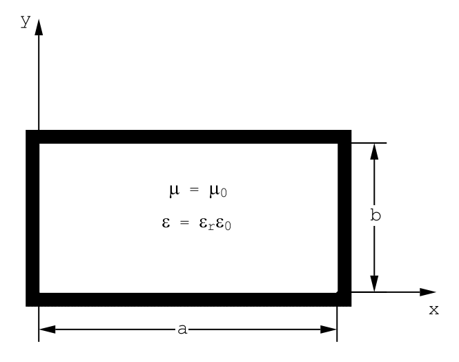
Furthermore, it is convenient at this point to change the description of the wave-guide co-ordinate system so that the origin is located at one corner of the hollow rectangular pipe as shown in Figure (12.2.4): in the new system the walls of the guide are formed by the intersection of the planes x=0,a and y=0,b. For a time variation of the form exp (−iωt) Maxwell’s equations become
curl(→E)=iωμ0→H,curl(→H)=−iωϵ→E.
The divergence of any curl is zero, and therefore the electric and the magnetic fields satisfy the conditions
div(→E)=0,div(→H)=0.
Note that the equations for →E and →H are very similar. This symmetry between the equations for →E and →H can be exploited to generate a second set of solutions to Maxwell’s equations from a primary set of fields that satisfy Maxwell’s equations. This works as follows: suppose that one has found the fields →E1 and →H1 that satisfy Equations (12.2.2). Now consider a second set of fields
→E2=Z→H1,→H2=−→E1/Z.
where Z=√μ0/ϵ is the wave impedance for a medium characterized by a permeability µ0 and a dielectric constant ϵ. Substitute these new fields into Equations (12.2.2) to obtain
curl(→E2)=iωμ0→H2.
Upon the substitution (12.2.6) this becomes
curl(→H1)=−iωμ0Z2→E1=−iωϵ→E1,
and this by hypothesis satisfies Maxwell’s Equations (12.2.2). Similarly, from (12.2.2) one has
curl(→H2)=−iωϵ→E2.
Upon substitution of Equations (12.2.6) one finds
curl(→E1)=iωμ0→H1,
so that the new fields, →E2 and →H2 satisfy both of Equations (12.2.2). Clearly Equations (12.2.4) are satisfied since →E2 and →H2 are proportional to →E1 and →H1. It follows that the prescription of Equation (12.2.6) can be used to generate a second, different, set of solutions for Maxwell’s equations from a primary set of solutions. This procedure can often be used to avoid a great deal of computational tedium.
12.2.1 TM Modes.
In order to proceed with the rectangular wave-guide problem it is convenient to use the vector potential →A, and the scalar potential, V, where
→H=curl(→A),→E=−grad(V)−μ0∂→A∂t.
The choice
Az=A(x,y)exp(i[kgz−ωt]),
plus Ax = Ay = 0 will guarantee that the z-component of the magnetic field, →H, is zero: in other words, this choice of vector potential will generate only TM modes, and
Hx=∂Az∂yHy=−∂Az∂x
For a time dependence exp (−iωt), and using (12.2.12) in Maxwell’s equations (12.2.2), one finds
curlcurl(→A)=ϵr(ωc)2→A+iωϵgrad(V).
But in cartesian co-ordinates
curlcurl(→A)=−∇2→A+graddiv(→A),
so that
∇2→A+ϵr(ωc)2→A=grad(div(→A)−iωϵV).
As explained in Chapter(7), one can set
iωϵV=div(→A),
so that for this problem where there are no driving charges or currents one finds
∇2→A+ϵr(ωc)2→A=0.
In particular, if →A has only a z-component one finds
∇2Az+ϵr(ωc)2Az=0,andiωϵV=∂Az∂z.
We require solutions that propagate along z: ie solutions that are proportional to exp (ikgz). Thus write
Az(x,y,z,t)=A(x,y)exp(i[kgz−ωt]),
for which A(x, y) must satisfy
∂2A∂x2+∂2A∂Y2−k2gA+ϵr(ωc)2A=0.
This equation is solved by products of sines and cosines:
A(x,y)= constant (sin(px) or cos(px))(sin(qy) or cos(qy)),
where
p2+q2+k2g=ϵr(ωc)2.
The particular combination of sines and cosines required must be chosen so that →H satisfies the boundary condition that the normal component of →H vanishes at the wave-guide walls. Using the magnetic field components calculated from Equation (12.2.12) and the co-ordinate system of Figure (12.2.4), it can be readily concluded that we require
A(x,y)=A0sin(mπxa)sin(nπyb),
so that
Hx=∂A∂y=(nπb)A0sin(mπxa)cos(nπyb),Hy=−∂A∂x=−(mπa)A0cos(mπxa)sin(nπyb),
where m,n are integers, and Equation (???) becomes
(mπa)2+(nπb)2+k2g=ϵr(ωc)2.
Notice that Az=0 at the walls of the wave-guide. Ez is proportional to Az so that if Az=0 on the walls of the guide then the tangential component Ez will also vanish on the walls of the wave-guide as is required by the boundary conditions on the tangential components of E.
The electric field components can be most easily calculated from the second of Equations (12.2.2),
curl(→H)=−iϵω→E.Ex=−iϵω(∂Hy∂z),Ey=+iϵω(∂Hx∂z),Ez=iϵω[∂Hy∂x−∂Hx∂y].
The resulting electric field components are (dropping the factor exp (i[kgz − ωt])):
Ex=−(mπa)(kgϵω)A0cos(mπxa)sin(nπyb),Ey=−(nπb)(kgϵω)A0sin(mπxa)cos(nπyb),Ez=(iϵω)[(mπa)2+(nπb)2]A0sin(mπxa)sin(nπyb).
Notice that these electric field components satisfy the requirement that the tangential components of E must vanish at the walls of the wave-guide. The field components Equations (12.2.28) and (12.2.32) correspond to the TMmn mode.
For a propagating wave the value of k2g calculated from (???) must be positive. This introduces a cut-off frequency, ωm, such that kg =0. This cut-off frequency is given by
ϵr(ωmc)2=(mπa)2+(nπb)2.
For given interior dimensions of the wave-guide there is a lower limit to the frequency for which a particular mode may be propagated along the waveguide. For example, a popular X-band wave-guide has interior dimensions a= 2.286 cm and b= 1.016 cm. For this guide the TM11 mode can be propagated only for frequencies greater than 16.15 GHz if ϵr= 1. There are no TM modes corresponding to m=0 or n=0 since the fields are zero if m=0 or if n=0 because A(x,y)=0 from Equation (???). Thus the lowest TM frequency that can be propagated down the above guide is 16.15 GHz.
Non-propagating TM modes do exist for frequencies less than the cutoff frequency. If ω < ωm then kg calculated from (???) is negative. This means that kg is a purely imaginary number, kg = iβ say. The phasor exp (i[kgz − ωt]) becomes exp (−βz) exp (−iωt) corresponding to a disturbance that decays to a small amplitude over a distance z ∼ (1/β).
12.2.2 TE Modes.
There exists another group of modes for which Ez = 0; these are the TE modes. Using the symmetry relations Equations (12.2.6) and the magnetic fields (12.2.28) one might guess that the TE mode electric fields ought to be given by (the factor exp (i[kgz − ωt]) is suppressed)
Ex=Z(nπb)A0sin(mπxa)cos(nπyb),Ey=−Z(mπa)A0cos(mπxa)sin(nπyb).
These electric fields satisfy Maxwell’s equations but they do not satisfy the boundary condition that the tangential components of →E must vanish at the wave-guide walls: ie. Ex=0 at y=0,b and Ey=0 at x=0,a (see Figure (12.2.4)). However, the following equations for the electric field components do satisfy the required boundary conditions:
Ex=E1cos(mπxa)sin(nπyb),Ey=E2sin(mπxa)cos(nπyb),Ez=0.
These field components vanish on the wave-guide walls. The electric field must also satisfy the Maxwell equation div(→E) = 0. This condition requires
∂Ex∂x+∂Eyy=0.
It follows that
(mπa)E1=−(nπb)E2.
Using this relation between E1 and E2 the electric field components corresponding to the TE modes in a rectangular wave-guide have the form:
Ex=(nπb)E0cos(mπxa)sin(nπyb),Ey=−(mπa)E0sin(mπxa)cos(nπyb),Ez=0,
where E0 is a constant, and the factor exp (i[kgz − ωt]) has again been suppressed. The magnetic field components corresponding to Equations (12.2.39) can be calculated from Faraday’s law: iωµ0 →H = curl(→E). The resulting field components are
Hx=+iωμ0∂Ey∂z=kgωμ0(mπa)E0sin(mπxa)cos(nπyb),Hy=−iωμ0∂Ex∂z=kgωμ0(nπb)E0cos(mπxa)sin(nπyb),Hz=−iωμ0(∂Ey∂x−∂Ex∂y)=iωμ0E0[(mπa)2+(nπb)2]cos(mπxa)cos(nπyb).
Eqns.(12.2.39) and (12.2.41) satisfy Maxwell’s equations and also the boundary conditions that the tangential components of →E and the normal components of →H vanish on the wave-guide walls. The TE10 mode discussed in section(12.1) corresponds to m=1,n=0: for this mode Ex = 0 and Hy = 0. Referring to the co-ordinate system of Figure (12.2.4) the field components for the TE10 mode are:
Ey=Asin(πxa)exp(i[kgz−ωt]),Hx=−kgωμ0Asin(πxa)exp(i[kgz−ωt]),Hz=−iωμ0(πa)Acos(πxa)exp(i[kgz−ωt]),
where A is a constant and
k2g=ϵr(ωc)2−(πa)2.
The cut-off frequency for this mode, corresponding to kg=0, is given by
ϵr(ωc)2=(πa)2.
For the popular X-band wave-guide used above for illustrative purposes one has a=2.286 cm and b=1.016 cm. For this guide, and ϵr = 1, the cut-of
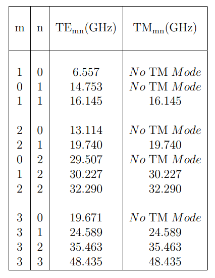
Table 12.2.1: Cut-off frequencies for the lowest transverse electric (TE) modes and the lowest transverse magnetic (TM) modes in X-band waveguides (RG52/U or WR90 brass guides). The internal dimensions of X-band waveguides are a= 0.900 inches = 2.286 cm, and b= 0.400 inches = 1.016 cm. The external dimensions of the guide are 1.00 x 0.50 inches. The cut-off frequencies were calculated for ϵr = 1 using (ωmnc)2=(mπa)2+(nπb)2.
frequency for the TE10 mode is 6.56 GHz. Cut-off frequencies for various modes in this X-band wave-guide are listed in Table(12.2.1). Notice that only one mode, the TE10 mode, can be propagated along this wave-guide for frequencies between 6.6 and 13.1 GHz.