
5.10: TM Reflection in Non-magnetic Media


- Last updated
- May 9, 2020
- Save as PDF

( \newcommand{\kernel}{\mathrm{null}\,}\)
Figure 5.10.1 shows a TM uniform plane wave incident on the planar boundary between two semi-infinite material regions.
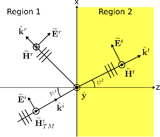 Figure 5.10.1: A transverse magnetic uniform plane wave obliquely incident on the planar boundary between two semi-infinite material regions. ( CC BY-SA 4.0; C. Wang)
In this case, the reflection coefficient is given by:
ΓTM=−η1cosψi+η2cosψt+η1cosψi+η2cosψt
where ψi and ψt are the angles of incidence and transmission (refraction), respectively; and η1 and η2 are the wave impedances in Regions 1 and 2, respectively. Many materials of practical interest are non-magnetic; that is, they have permeability that is not significantly different from the permeability of free space. In this section, we consider the behavior of the reflection coefficient for this class of materials.
To begin, recall the general form of Snell’s law:
sinψt=β1β2sinψi
In non-magnetic media, the permeabilities μ1 and μ2 are assumed equal to μ0. Thus:
β1β2=ω√μ1ϵ1ω√μ2ϵ2=√ϵ1ϵ2
Since permittivity ϵ can be expressed as ϵ0 times the relative permittivity ϵr, we may reduce further to:
β1β2=√ϵr1ϵr2
Now Equation ??? reduces to:
sinψt=√ϵr1ϵr2sinψi
Next, note that for any value ψ, one may write cosine in terms of sine as follows:
cosψ=√1−sin2ψ
Therefore,
cosψt=√1−ϵr1ϵr2sin2ψi
Also we note that in non-magnetic media
η1=√μ1ϵ1=√μ0ϵr1ϵ0=η0√ϵr1η2=√μ2ϵ2=√μ0ϵr2ϵ0=η0√ϵr2
where η0 is the wave impedance in free space. Making substitutions into Equation ???, we obtain:
ΓTM=−(η0/√ϵr1)cosψi+(η0/√ϵr2)cosψt+(η0/√ϵr1)cosψi+(η0/√ϵr2)cosψt
Multiplying numerator and denominator by √ϵr2/η0, we obtain:
ΓTM=−√ϵr2/ϵr1cosψi+cosψt+√ϵr2/ϵr1cosψi+cosψt
Substituting Equation ???, we obtain:
ΓTM=−√ϵr2/ϵr1cosψi+√1−(ϵr1/ϵr2)sin2ψi+√ϵr2/ϵr1cosψi+√1−(ϵr1/ϵr2)sin2ψi
This expression has the advantage that it is now entirely in terms of ψi, with no need to first calculate ψt.
Finally, multiplying numerator and denominator by √ϵr2/ϵr1, we obtain:
ΓTM=−(ϵr2/ϵr1)cosψi+√ϵr2/ϵr1−sin2ψi+(ϵr2/ϵr1)cosψi+√ϵr2/ϵr1−sin2ψi
Using Equation ???, we can easily see how different combinations of material affect the reflection coefficient. First, we note that when ϵr1=ϵr2 (i.e., same media on both sides of the boundary), ΓTM=0 as expected. When ϵr1>ϵr2 (e.g., wave traveling in glass toward air), we see that it is possible for ϵr2/ϵr1−sin2ψi to be negative, which makes ΓTM complex-valued. This results in total internal reflection, and is addressed in another section. When ϵr1<ϵr2 (e.g., wave traveling in air toward glass), we see that ϵr2/ϵr1−sin2ψi is always positive, so ΓTM is always real-valued.
Let us continue with the ϵr1<ϵr2 condition. Figure 5.10.2 shows ΓTM plotted for various combinations of media over all possible angles of incidence from 0 (normal incidence) to π/2 (grazing incidence).
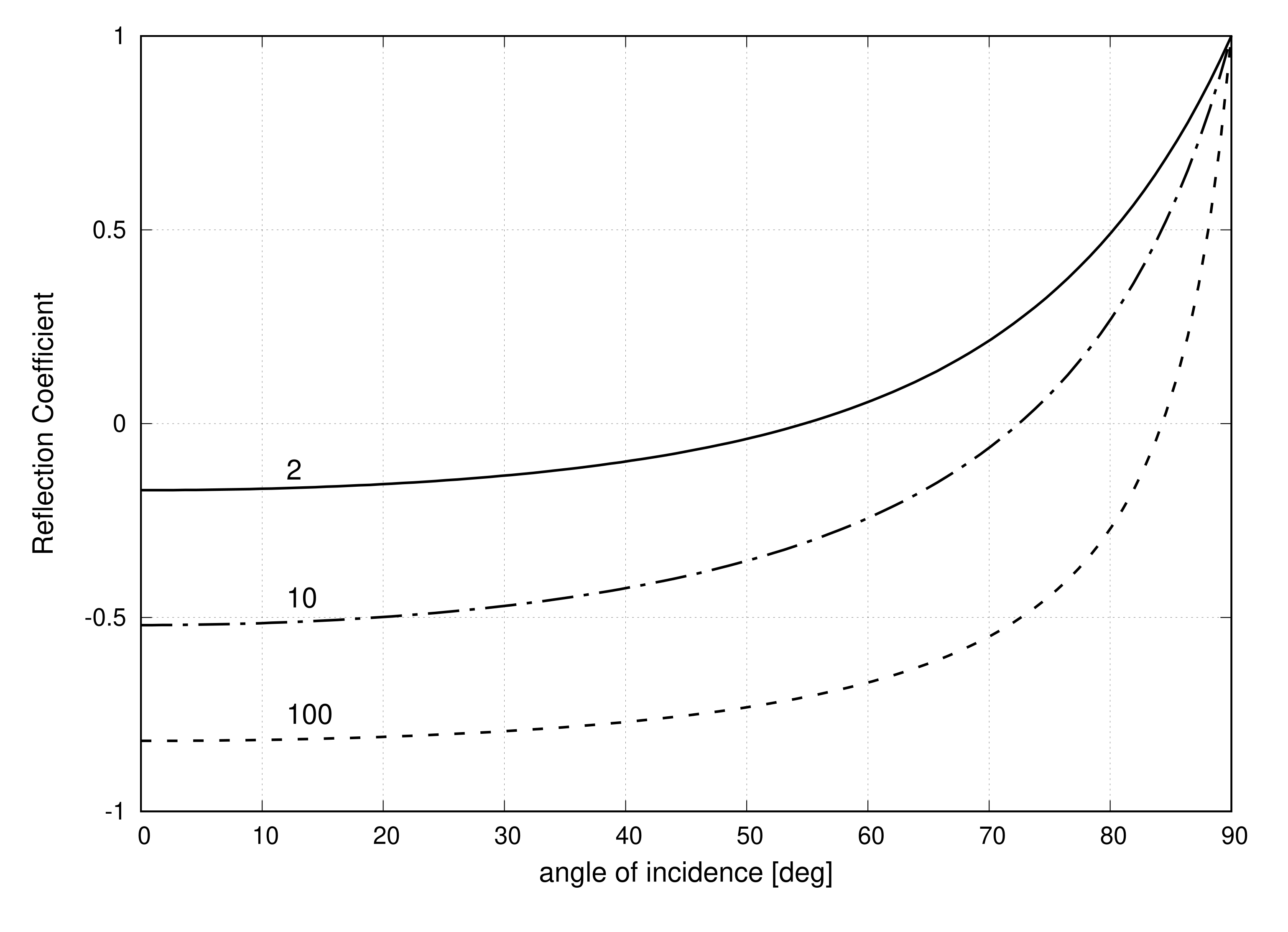 Figure 5.10.2: The reflection coefficient ΓTM as a function of angle of incidence ψi for various media combinations, parameterized as ϵr2/ϵr1.
We observe:
In non-magnetic media with ϵr1<ϵr2, ΓTM is real-valued and increases from a negative value for normal incidence to +1 as ψi approaches grazing incidence.
Note that at any particular angle of incidence, ΓTM trends toward −1 as ϵr2/ϵr1→∞. In this respect, the behavior of the TM component is similar to that of the TE component. In other words: As ϵr2/ϵr1→∞, the result for both the TE and TM components are increasingly similar to the result we would obtain for a perfect conductor in Region 2.
Also note that when ϵr1<ϵr2, ΓTM changes sign from negative to positive as angle of incidence increases from 0 to π/2. This behavior is quite different from that of the TE component, which is always negative for ϵr1<ϵr2. The angle of incidence at which ΓTM=0 is referred to as Brewster’s angle, which we assign the symbol ψiB. Thus:
ψiB≜ψi at which ΓTM=0
In the discussion that follows, here is the key point to keep in mind:
Brewster’s angle ψiB is the angle of incidence at which ΓTM=0.
Brewster’s angle is also referred to as the polarizing angle. The motivation for the term “polarizing angle” is demonstrated in Figure 5.10.3.
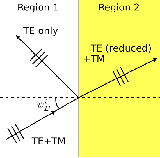 Figure 5.10.3: Reflection of a plane wave with angle of incidence ψi equal to the polarizing angle ψiB. Here the media are non-magnetic with ϵr1<ϵr2. ( CC BY-SA 4.0; C. Wang)
In this figure, a plane wave is incident with ψi=ψiB. The wave may contain TE and TM components in any combination. Applying the principle of superposition, we may consider these components separately. The TE component of the incident wave will scatter as reflected and transmitted waves which are also TE. However, ΓTM=0 when ψi=ψiB, so the TM component of the transmitted wave will be TM, but the TM component of the reflected wave will be zero. Thus, the total (TE+TM) reflected wave will be purely TE, regardless of the TM component of the incident wave. This principle can be exploited to suppress the TM component of a wave having both TE and TM components. This method can be used to isolate the TE and TM components of a wave.
Derivation of a formula for Brewster’s angle
Brewster’s angle for any particular combination of non-magnetic media may be determined as follows. ΓTM=0 when the numerator of Equation ??? equals zero, so:
−RcosψiB+√R−sin2ψiB=0
where we have made the substitution R≜ϵr2/ϵr1 to improve clarity. Moving the second term to the right side of the equation and squaring both sides, we obtain:
R2cos2ψiB=R−sin2ψiB
Now employing a trigonometric identity on the left side of the equation, we obtain:
R2(1−sin2ψiB)=R−sin2ψiBR2−R2sin2ψiB=R−sin2ψiB(1−R2)sin2ψiB=R−R2
and finally
sinψiB=√R−R21−R2
Although this equation gets the job done, it is possible to simplify further. Note that Equation ??? can be interpreted as a description of the right triangle shown in Figure 5.10.4.
 Figure 5.10.4: Derivation of a simple formula for Brewster's angle for non-magnetic media. ( CC BY-SA 4.0; C. Wang)
In the figure, we have identified the length h of the vertical side and the length d of the hypotenuse as:
h≜√R−R2d≜√1−R2
The length b of the horizontal side is therefore
b=√d2−h2=√1−R
Subsequently, we observe
tanψiB=hb=√R−R2√1−R=√R
Thus, we have found
tanψiB=√ϵr2ϵr1
A plane wave is incident from air onto the planar boundary with a glass region. The glass exhibits relative permittivity of 2.1. The incident wave contains both TE and TM components. At what angle of incidence ψi will the reflected wave be purely TE?
Solution
Using Equation ???:
tanψiB=√ϵr2ϵr1=√2.11≅1.449
Therefore, Brewster’s angle is ψiB≅55.4∘. This is the angle ψi at which ΓTM=0. Therefore, when ψi=ψiB, the reflected wave contains no TM component and therefore must be purely TE.