3.5: Two-element circuits and RLC resonators

Two-element circuits and uncoupled RLC resonators

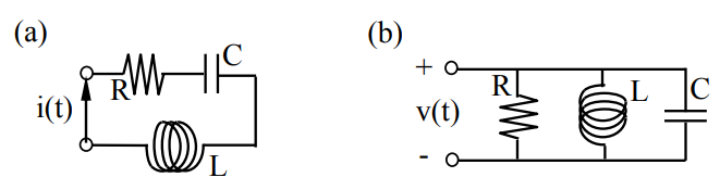
RLC resonators typically consist of a resistor R, inductor L, and capacitor C connected in series or parallel, as illustrated in Figure 3.5.1. RLC resonators are of interest because they behave much like other electromagnetic systems that store both electric and magnetic energy, which slowly dissipates due to resistive losses. First we shall find and solve the differential equations that characterize RLC resonators and their simpler sub-systems: RC, RL, and LC circuits. This will lead to definitions of resonant frequency ω_o and Q, which will then be related in Section 3.5.2 to the frequency response of RLC resonators that are coupled to circuits.

Figure \(\PageIndex{1}\): Series and parallel RLC resonators.

The differential equations that govern the voltages across R’s, L’s, and C’s are, respectively:

\[ \mathrm{v}_{\mathrm{R}}=\mathrm{iR}\]

\[\mathrm{v}_{\mathrm{L}}=\mathrm{L} \ \mathrm{di} / \mathrm{dt}\]

\[\mathrm{v}_{\mathrm{C}}=(1 / \mathrm{C}) \int \mathrm{i} \ \mathrm{d} \mathrm{t}\]

Kirchoff’s voltage law applied to the series RLC circuit of Figure 3.5.1(a) says that the sum of the voltages (3.5.1), (3.5.2), and (3.5.3) is zero:

\[\mathrm{d}^{2} \mathrm{i} / \mathrm{dt}^{2}+(\mathrm{R} / \mathrm{L}) \mathrm{di} / \mathrm{dt}+(1 / \mathrm{LC}) \mathrm{i}=0 \]

where we have divided by L and differentiated to simplify the equation. Before solving it, it is useful to solve simpler versions for RC, RL, and LC circuits, where we ignore one of the three elements.

In the RC limit where L = 0 we add (3.5.1) and (3.5.3) to yield the differential equation:

\[ \mathrm{di} / \mathrm{dt}+(1 / \mathrm{RC}) \mathrm{i}=0\]

This says that i(t) can be any function with the property that the first derivative is the same as the original signal, times a constant. This property is restricted to exponentials and their sums, such as sines and cosines. Let's represent i(t) by I_oe^st, where:

\[\mathrm{i}(\mathrm{t})=\mathrm{R}_{\mathrm{e}}\left\{\mathrm{I}_{\mathrm{o}} \mathrm{e}^{\mathrm{st}}\right\}\]

where the complex frequency s is:

\[\mathrm{s} \equiv \alpha+\mathrm{j} \omega\]

We can substitute (3.5.6) into (3.5.5) to yield:

\[\operatorname{Re}\left\{[\mathrm{s}+(1 / \mathrm{RC})] \mathrm{I}_{0} \mathrm{e}^{\mathrm{st}}\right\}=0\]

Since e^st is not always zero, to satisfy (3.5.8) it follows that s = - 1/RC and:

\[\mathrm{i}(\mathrm{t})=\mathrm{I}_{\mathrm{o}} \mathrm{e}^{-(1 / \mathrm{RC}) \mathrm{t}}=\mathrm{I}_{\mathrm{o}} \mathrm{e}^{-\mathrm{t} / \tau} \qquad\qquad\qquad \text{(RC current response)}\]

where \(\tau\) equals RC seconds and is the RC time constant. I_o is chosen to satisfy initial conditions, which were not given here.

A simple example illustrates how initial conditions can be incorporated in the solution. We simply need as many equations for t = 0 as there are unknown variables. In the present case we need one equation to determine I_o. Suppose the RC circuit [of Figure 3.5.1(a) with L = 0] was at rest at t = 0, but the capacitor was charged to V_o volts. Then we know that the initial current I_o at t = 0 must be V_o/R.

In the RL limit where C = ∞ we add (3.5.1) and (3.5.2) to yield di/dt + (R/L)i = 0, which has the same form of solution (3.5.6), so that s = -R/L and:

\[\mathrm{i}(\mathrm{t})=\mathrm{I}_{\mathrm{o}} \mathrm{e}^{-(\mathrm{R} / \mathrm{L}) \mathrm{t}}=\mathrm{I}_{\mathrm{o}} \mathrm{e}^{-\mathrm{t} / \tau} \qquad\qquad\qquad \text{(RL current response) }\]

where the RL time constant \(\tau\) is L/R seconds.

In the LC limit where R = 0 we add (3.5.2) and (3.5.3) to yield:

\[\mathrm{d}^{2} \mathrm{i} / \mathrm{dt}^{2}+(1 / \mathrm{LC}) \mathrm{i}=0\]

Its solution also has the form (3.5.6). Because i(t) is real and e^jωt is complex, it is easier to assume sinusoidal solutions, where the phase φ and magnitude I_o would be determined by initial conditions. This form of the solution would be:

\[\mathrm{i}(\mathrm{t})=\mathrm{I}_{\mathrm{o}} \cos \left(\omega_{\mathrm{o}} \mathrm{t}+\phi\right) \qquad\qquad\qquad \text{(LC current response)}\]

where ω_o = 2\(\pi\)f_o is found by substituting (3.5.12) into (3.5.11) to yield [ω_o² – (LC)^-1]i(t) = 0, so:

\[\omega_{\mathrm{o}}=\frac{1}{\sqrt{\mathrm{L} C}} \ \left[\text { radians } \mathrm{s}^{-1}\right] \qquad \qquad \qquad \text{ (LC resonant frequency) }\]

We could alternatively express this solution (3.5.12) as the sum of two exponentials using the identity \(\cos \omega t \equiv\left(e^{j \omega t}+e^{-j \omega t}\right) / 2\).

RLC circuits exhibit both oscillatory resonance and exponential decay. If we substitute the generic solution \(\underline{I}_{0} \mathrm{e}^{\mathrm{st}}\) (3.5.6) into the RLC differential equation (3.5.4) for the series RLC resonator of Figure 3.5.1(a) we obtain:

\[\left(s^{2}+s R / L+1 / L C\right) \underline{I}_{0} e^{s t}=\left(s-s_{1}\right)\left(s-s_{2}\right) \underline{I}_{0} e^{s t}=0\]

The RLC resonant frequencies s₁ and s₂ are solutions to (3.5.14) and can be found by solving this quadratic equation⁹ to yield:

\[\mathrm{s}_{\mathrm{i}}=-\mathrm{R} / 2 \mathrm{L} \pm \mathrm{j}\left[(1 / \mathrm{LC})-(\mathrm{R} / 2 \mathrm{L})^{2}\right]^{0.5} \qquad \qquad \qquad \text{(series RLC resonant frequencies) }\]

When R = 0 this reduces to the LC resonant frequency solution (3.5.13).

⁹ A quadratic equation in x has the form ax² + bx + c = 0 and the solution x = (-b ± [b² - 4ac]^0.5)/2a.

The generic solution \( \mathrm{i}(\mathrm{t})=\mathrm{\underline{I}}_{\mathrm{o}}^{\prime} \mathrm{e}^{\mathrm{st}}\) is complex, where \(\underline{I}_{0}^{\prime} \equiv \mathrm{I}_{0} \mathrm{e}^{\mathrm{j} \phi} \):

\[\mathrm{i}(\mathrm{t})=\mathrm{R}_{\mathrm{e}}\left\{\mathrm{\underline{I}}_{\mathrm{o}}^{\prime} \mathrm{e}^{\mathrm{s}_{1} \mathrm{t}}\right\}=\mathrm{R}_{\mathrm{e}}\left\{\mathrm{I}_{\mathrm{o}} \mathrm{e}^{\mathrm{j} \phi} \mathrm{e}^{-(\mathrm{R} / 2 \mathrm{L}) \mathrm{t}} \mathrm{t}^{\mathrm{j} \omega \mathrm{t}}\right\}=\mathrm{I}_{\mathrm{o}} \mathrm{e}^{-(\mathrm{R} / 2 \mathrm{L}) \mathrm{t}} \cos (\omega \mathrm{t}+\phi)\]

where \( \omega=\left[(\mathrm{LC})^{-1}+(\mathrm{R} / 2 \mathrm{L})^{2}\right]^{0.5} \cong(\mathrm{LC})^{-0.5}\). I_o and φ can be found from the initial conditions, which are the initial current through L and the initial voltage across C, corresponding to the initial energy storage terms. If we choose the time origin so that the phase φ = 0, the instantaneous magnetic energy stored in the inductor (3.2.23) is:

\[\mathrm{w}_{\mathrm{m}}(\mathrm{t})=\mathrm{Li}^{2} / 2=\left(\mathrm{LI}_{\mathrm{o}}^{2} / 2\right) \mathrm{e}^{-\mathrm{R} t / \mathrm{L}} \cos ^{2} \omega \mathrm{t}=\left(\mathrm{LI}_{\mathrm{o}}^{2} / 4\right) \mathrm{e}^{-\mathrm{R} t / \mathrm{L}}(1+\cos 2 \omega \mathrm{t})\]

Because w_m = 0 twice per cycle and energy is conserved, the peak electric energy w_e(t) stored in the capacitor must be intermediate between the peak magnetic energies stored in the inductor (e^Rt/LLI_o² /2) during the preceding and following cycles. Also, since dv_C/dt = i/C, the cosine variations of i(t) produce a sinusoidal variation in the voltage v_C(t) across the capacitor. Together these two facts yield: \( \mathrm{w}_{\mathrm{e}}(\mathrm{t}) \cong\left(\mathrm{LI}_{\mathrm{o}}^{2} / 2\right) \mathrm{e}^{-\mathrm{R} t / \mathrm{L}} \sin ^{2} \omega \mathrm{t}\). If we define Vo as the maximum initial voltage corresponding to the maximum initial current I_o, and recall the expression (3.1.16) for w_e(t), we find:

\[ \mathrm{w}_{\mathrm{e}}(\mathrm{t})=\mathrm{Cv}^{2} / 2 \cong\left(\mathrm{CV}_{\mathrm{o}}^{2} / 2\right) \mathrm{e}^{-\mathrm{R} t / \mathrm{L}} \sin ^{2} \omega \mathrm{t}=\left(\mathrm{CV}_{\mathrm{o}}^{2} / 4\right) \mathrm{e}^{-\mathrm{R} t / \mathrm{L}}(1-\cos 2 \omega \mathrm{t})\]

Comparison of (3.5.17) and (3.5.18) in combination with conservation of energy yields:

\[ \mathrm{V}_{\mathrm{o}} \cong(\mathrm{L} / \mathrm{C})^{0.5} \mathrm{I}_{\mathrm{o}}\]

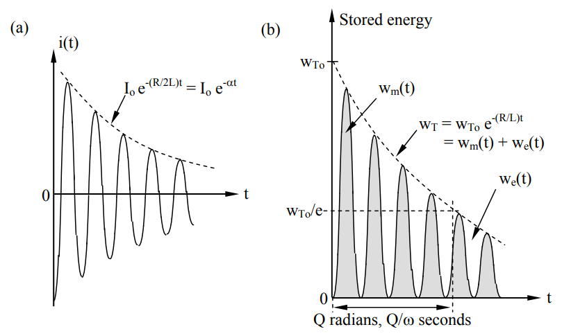
Figure 3.5.2 illustrates how the current and energy storage decays exponentially with time while undergoing conversion between electric and magnetic energy storage at 2ω radians s^-1; the time constant for current and voltage is \(\tau\) = 2L/R seconds, and that for energy is L/R.

One useful way to characterize a resonance is by the dimensionless quantity Q, which is the number of radians required before the total energy w_T decays to 1/e of its original value, as illustrated in Figure 3.5.2(b). That is:

\[\mathrm{w}_{\mathrm{T}}=\mathrm{w}_{\mathrm{To}} \mathrm{e}^{-2 \alpha \mathrm{t}}=\mathrm{w}_{\mathrm{To}} \mathrm{e}^{-\omega \mathrm{t} / \mathrm{Q}} \ [\mathrm{J}]\]

The decay rate \(\alpha\) for current and voltage is therefore simply related to Q:

\[ \alpha=\omega / 2 \mathrm{Q}\]

Figure \(\PageIndex{2}\): Time variation of current and energy storage in RLC circuits.

If we find the power dissipated P_d [W] by differentiating total energy w_T with respect to time using (3.5.20), we can then derive a common alternative definition for Q:

\[\mathrm{P}_{\mathrm{d}}=-\mathrm{d} \mathrm{w}_{\mathrm{T}} / \mathrm{dt}=(\omega / \mathrm{Q}) \mathrm{w}_{\mathrm{T}}\]

\[\mathrm{Q}=\omega \mathrm{w}_{\mathrm{T}} / \mathrm{P}_{\mathrm{d}} \qquad\qquad\qquad \text{(one definition of Q) }\]

For the series RLC resonator \(\alpha\) = R/2L and ω ≅ (LC)^-0.5, so (3.5.21) yields:

\[\mathrm{Q}=\omega / 2 \alpha=\omega \mathrm{L} / \mathrm{R} \cong(\mathrm{L} / \mathrm{C})^{0.5} / \mathrm{R} \qquad\qquad\qquad \text{(Q of series RLC resonator) }\]

Figure 3.5.1(b) illustrates a parallel RLC resonator. KCL says that the sum of the currents into any node is zero, so:

\[\mathrm{C} \ \mathrm{dv} / \mathrm{dt}+\mathrm{v} / \mathrm{R}+(1 / \mathrm{L}) \int \mathrm{v} \ \mathrm{dt}=0\]

\[\mathrm{d}^{2} \mathrm{v} / \mathrm{dt}^{2}+(1 / \mathrm{RC}) \mathrm{dv} / \mathrm{dt}+(1 / \mathrm{LC}) \mathrm{v}=0\]

If v = V_oe^st, then:

\[\left[s^{2}+(1 / R C) s+(L / C)\right]=0\]

\[\mathrm{s}=-(1 / 2 \mathrm{RC}) \pm \mathrm{j}\left[(1 / \mathrm{LC})-(1 / 2 \mathrm{RC})^{2}\right]^{0.5} \qquad \qquad \qquad \text{(parallel RLC resonance) }\]

Analogous to (3.5.16) we find:

\[\mathrm{v}(\mathrm{t})=\mathrm{R}_{\mathrm{e}}\left\{\underline{\mathrm{V}}_{\mathrm{o}}^{\prime} \mathrm{e}^{\mathrm{s}_{1} \mathrm{t}}\right\}=\mathrm{V}_{\mathrm{o}} \mathrm{e}^{-(1 / 2 \mathrm{R} \mathrm{C}) \mathrm{t}} \cos (\omega \mathrm{t}+\phi) \]

where \( \underline{V}_{0}^{\prime}=V_{0} e^{j \phi}\). It follows that for a parallel RLC resonator:

\[\omega=\left[(\mathrm{LC})^{-1}-(2 \mathrm{RC})^{-2}\right]^{0.5} \cong(\mathrm{LC})^{-0.5}\]

\[Q=\omega / 2 \alpha=\omega R C=R(C / L)^{0.5} \qquad \qquad \qquad \text{(Q of parallel RLC resonator) }\]

Example \(\PageIndex{A}\)

What values of L and C would give a parallel resonator at 1 MHz a Q of 100 if R = 10⁶/2\(\pi\)?

Solution

LC = 1/ω_o² = 1/(2\(\pi\)10⁶)² , and Q = 100 = ωRC = 2\(\pi\)10⁶(10⁶/2\(\pi\))C so C = 10^-10 [F] and L = 1/ω_o² c ≅ 2.5×10^-4 [Hy].

Coupled RLC resonators

RLC resonators are usually coupled to an environment that can be represented by either its Thevenin or Norton equivalent circuit, as illustrated in Figure 3.5.3(a) and (b), respectively, for purely resistive circuits.

Figure \(\PageIndex{3}\): Series and parallel RLC resonators driven by Thevenin and Norton equivalent circuits.

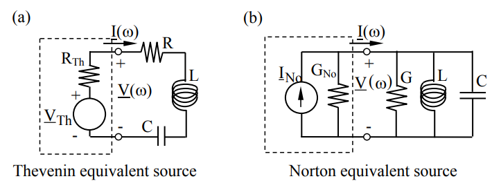
A Thevenin equivalent consists of a voltage source V_Th in series with an impedance \(\underline{Z}_{\mathrm{Th}}=\mathrm{R}_{\mathrm{Th}}+\mathrm{jX}_{\mathrm{Th}}\), while a Norton equivalent circuit consists of a current source I_No in parallel with an admittance \(\underline{Y}_{\mathrm{No}}=\mathrm{G}_{\mathrm{No}}+\mathrm{jU}_{\mathrm{No}}\). The Thevenin equivalent of a resistive Norton equivalent circuit has open-circuit voltage V_Th = I_No/G_No, and R_Th = 1/G_No; that is, their opencircuit voltages, short-circuit currents, and impedances are the same. No single-frequency electrical experiment performed at the terminals can distinguish ideal linear circuits from their Thevenin or Norton equivalents.

An important characteristic of a resonator is the frequency dependence of its power dissipation. If R_Th = 0, the series RLC resonator of Figure 3.5.3(a) dissipates:

\[\mathrm{P}_{\mathrm{d}}=\mathrm{R}|\mathrm{\underline{I}}|^{2} / 2[\mathrm{W}]\]

\[P_{d}=\left[R\left|\underline{V}_{T h}\right|^{2} / 2\right] /\left|R+L s+C^{-1} s^{-1}\right|^{2}=\left[R\left|\underline{V}_{T h}\right|^{2} / 2\right]|s / L|^{2} /\left|\left(s-s_{1}\right)\left(s-s_{2}\right)\right|^{2}\]

where s₁ and s₂ are given by (3.5.15):

\[\mathrm{s}_{\mathrm{i}}=-\mathrm{R} / 2 \mathrm{L} \pm \mathrm{j}\left[(1 / \mathrm{LC})-(\mathrm{R} / 2 \mathrm{L})^{2}\right]^{0.5}=-\alpha \pm \mathrm{j} \omega_{\mathrm{o}}^{\prime} \qquad\qquad\qquad \text { (series RLC resonances) }\]

The maximum value of Pd is achieved when ω ≅ ω′_o :

\[P_{\mathrm{d} \max }=\left|\underline{\mathrm{V}}_{\mathrm{Th}}\right|^{2} / 2 \mathrm{R}\]

This simple expression is expected since the reactive impedances of L and C cancel at ω_o, leaving only R.

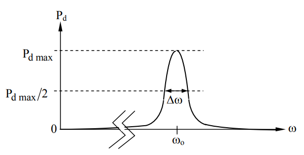
If \((1 / \mathrm{LC}) \gg(\mathrm{R} / 2 \mathrm{L})\) so that \(\omega_{\mathrm{o}} \cong \omega_{\mathrm{o}}^{\prime}\), then as ω - ω_o increases from zero to \(\alpha\), |s − s₁ | = | jω_o − (jω_o + \(\alpha\)) | increases from \(\alpha\) to \(\sqrt{2} \alpha\). This departure from resonance approximately doubles the denominator of (3.5.33) and halves P_d. As ω departs still further from ωo and resonance, P_d eventually approaches zero because the impedances of L and C approach infinity at infinite and zero frequency, respectively. The total frequency response Pd(f) of this series RLC resonator is suggested in Figure 3.5.4. The resonator bandwidth or half-power bandwidth Δω is said to be the difference between the two half-power frequencies, or Δω ≅ 2\(\alpha\) = R/L for this series circuit. Δω is simply related to ω_o and Q for both series and parallel resonances, as follows from (3.5.21):

\[\mathrm{Q}=\omega_{\mathrm{o}} / 2 \alpha=\omega_{\mathrm{o}} / \Delta \omega \qquad \qquad \qquad \text{(Q versus bandwidth) }\]

Parallel RLC resonators behave similarly except that:

\[ \mathrm{s}_{\mathrm{i}}=-\mathrm{G} / 2 \mathrm{L} \pm \mathrm{j}\left[(1 / \mathrm{LC})-(\mathrm{G} / 2 \mathrm{L})^{2}\right]^{0.5}=-\alpha \pm \mathrm{j} \omega_{\mathrm{o}}^{\prime} \qquad\qquad\qquad \text{(parallel RLC resonances) }\]

where R, L, and C in (3.5.34) have been replaced by their duals G, C, and L, respectively.

Figure \(\PageIndex{4}\): RLC power dissipation near resonance.

Resonators reduce to their resistors at resonance because the impedance of the LC portion approaches zero or infinity for series or parallel resonators, respectively. At resonance P_d is maximized when the source R_s and load R resistances match, as is easily shown by setting the derivative dP_d/dR = 0 and solving for R. In this case we say the resonator is critically matched to its source, for all available power is then transferred to the load at resonance.

This critically matched condition can also be related to the Q’s of a coupled resonator with zero Thevenin voltage applied from outside, where we define internal Q (or Q_I) as corresponding to power dissipated internally in the resonator, external Q (or Q_E) as corresponding to power dissipated externally in the source resistance, and loaded Q (or Q_L) as corresponding to the total power dissipated both internally (P_DI) and externally (P_DE). That is, following (3.5.23):

\[\mathrm{Q}_{\mathrm{I}} \equiv \omega \mathrm{w}_{\mathrm{T}} / \mathrm{P}_{\mathrm{DI}} \qquad\qquad\qquad \text{(internal Q) }\]

\[\mathrm{Q}_{\mathrm{E}} \equiv \omega \mathrm{w}_{\mathrm{T}} / \mathrm{P}_{\mathrm{DE}} \qquad\qquad\qquad \text{(external Q) }\]

\[\mathrm{Q}_{\mathrm{L}} \equiv \omega \mathrm{w}_{\mathrm{T}} /\left(\mathrm{P}_{\mathrm{DI}}+\mathrm{P}_{\mathrm{DE}}\right) \qquad \qquad \qquad \text{(loaded Q)}\]

Therefore these Q’s are simply related:

\[\mathrm{Q}_{\mathrm{L}}^{-1}=\mathrm{Q}_{\mathrm{I}}^{-1}+\mathrm{Q}_{\mathrm{E}}^{-1}\]

It is Q_L that corresponds to Δω for coupled resonators (Q_L = ω_o/Δω) .

For example, by applying Equations (3.5.38–40) to a series RLC resonator, we readily obtain:

\[Q_{I}=\omega_{0} L / R\]

\[\mathrm{Q}_{\mathrm{E}}=\omega_{\mathrm{o}} \mathrm{L} / \mathrm{R}_{\mathrm{Th}}\]

\[Q_{L}=\omega_{0} L /\left(R_{T h}+R\right)\]

For a parallel RLC resonator the Q’s become:

\[\mathrm{Q}_{\mathrm{I}}=\omega_{\mathrm{o}} \mathrm{RC}\]

\[\mathrm{Q}_{\mathrm{E}}=\omega_{\mathrm{O}} \mathrm{R}_{\mathrm{Th}} \mathrm{C}\]

\[\mathrm{Q}_{\mathrm{L}}=\omega_{\mathrm{o}} \mathrm{CR}_{\mathrm{Th}} \mathrm{R} /\left(\mathrm{R}_{\mathrm{Th}}+\mathrm{R}\right)\]

Since the source and load resistances are matched for maximum power dissipation at resonance, it follows from Figure 3.5.3 that a critically coupled resonator or matched resonator results when Q_I = Q_E. These expressions for Q are in terms of energies stored and power dissipated, and can readily be applied to electromagnetic resonances of cavities or other structures, yielding their bandwidths and conditions for maximum power transfer to loads, as discussed in Section 9.4.