10.3: Antenna gain, effective area, and circuit properties

Antenna directivity and gain

The far-field intensity \( \overline{\mathrm{P}}(\mathrm{r}, \theta)\) [W m^-2] radiated by any antenna is a function of direction, as given for a short dipole antenna by (10.2.27) and illustrated in Figure 10.2.4. Antenna gain G(θ,φ) is defined as the ratio of the intensity P(θ,φ,r) to the intensity [Wm^-2] that would result if the same total power available at the antenna terminals, P_A [W], were radiated isotropically over 4π steradians. G(θ,φ) is often called “gain over isotropic” where:

\[\mathrm{G}(\theta, \phi) \equiv \frac{\mathrm{P}(\mathrm{r}, \theta, \phi)}{\left(\mathrm{P}_{\mathrm{A}} / 4 \pi \mathrm{r}^{2}\right)} \qquad \qquad \qquad \text{(antenna gain definition) }\]

A related quantity is antenna directivity D(θ,φ), which is normalized to the total power radiated P_T rather than to the power P_A available at the antenna terminals:

\[\mathrm{D}(\theta, \phi) \equiv \frac{\mathrm{P}(\mathrm{r}, \theta, \phi)}{\left(\mathrm{P}_{\mathrm{T}} / 4 \pi \mathrm{r}^{2}\right)} \qquad \qquad \qquad \text{(antenna directivity definition)}\]

The transmitted power is less than the available power if the antenna is mismatched or lossy. Since the total power radiated is \( \mathrm{P}_{\mathrm{T}}=\mathrm{r}^{2} \int_{4 \pi} \mathrm{P}(\mathrm{r}, \theta, \phi) \sin \theta \mathrm{d} \theta \mathrm{d} \phi\), a useful relation follows from (10.3.2):

\[\oint_{4 \pi} \mathrm{D}(\theta, \phi) \sin \theta \mathrm d \theta \mathrm d \phi=4 \pi \]

Equation (10.3.3) says that if the directivity or gain is large in one direction, it must be correspondingly diminished elsewhere, as suggested in Figure 10.2.4, where the pattern is plotted relative to an isotropic radiator and exhibits its “main lobe” in the direction θ = 90°. This pattern is independent of φ. The half-power antenna beamwidth in the θ direction is the angle θ_B between two directions where the radiated power is half that radiated at the peak, as illustrated. Thus (10.3.3) and the figure also suggest that high directivity antennas have narrower beamwidths θ_B, or are more “directive”.

The ratio P_T/P_A is that fraction of the power available at the antenna terminals (P_A) that is radiated; it is defined as the radiation efficiency \(\eta_{\mathrm{R}} \):

\[\eta_{\mathrm{R}} \equiv \mathrm{P}_{\mathrm{T}} / \mathrm{P}_{\mathrm{A}} \qquad \qquad \qquad \text{(radiation efficiency)}\]

\[\mathrm{G}(\theta, \phi) \equiv \eta_{\mathrm{R}} \mathrm{D}(\theta, \phi)\]

The radiation efficiency is usually near unity because the resistive losses and the reflective losses due to impedance mismatches are small in most systems. Typical exceptions to the rule \(\eta_{\mathrm{R}} \cong 1 \) include most short dipoles and antennas that are used over bandwidths much greater than an octave; their impedances are difficult to match.

The directivity of a short dipole antenna is given by substituting (10.2.27) and (10.2.28) into (10.3.2):

\[\mathrm{D}(\theta, \phi)=\frac{\left(\eta_{\mathrm{o}} / 2\right)\left|\mathrm{\underline I}_{\mathrm{o}} \mathrm{d} / \lambda 2 \mathrm{r}\right|^{2} \sin ^{2} \theta}{\left(\eta_{\mathrm{o}} \pi / 3\right)\left|\mathrm{\underline I}_{\mathrm{o}} \mathrm{d} / \lambda\right|^{2} / 4 \pi \mathrm{r}^{2}}=1.5 \sin ^{2} \theta \qquad\qquad\qquad(\text { short dipole directivity })\]

Lossless matched short dipole antennas have gain:

\[\mathrm{G}(\theta, \phi)=1.5 \sin ^{2} \theta \qquad \qquad \qquad \text{(short-dipole antenna gain) }\]

Example \(\PageIndex{A}\)

What is the maximum solid angle \(\Omega_{\mathrm{B}}\) [steradians] over which a lossless matched antenna can have constant gain G_o = 40 dB? If the beam is circular, approximately what is its diameter θ_B? How much transmitter power P_T is required to yield \(\underline{\mathrm E}_{0}=1 \) volt per meter at 10 kilometers?

Solution

Since G(θ,φ) = D(θ,φ) for a lossless matched antenna, and \(\int_{4 \pi} \mathrm{D}(\theta, \phi) \mathrm{d} \Omega=4 \pi \), it follows that \(\mathrm{G}_{\mathrm{o}} \Omega_{\mathrm{B}}=4 \pi \) since the maximum gain results when all sidelobes have G = 0. Therefore \( \Omega_{\mathrm{B}}=4 \pi \times 10^{-4}\), corresponding to \( \pi \theta_{\mathrm{B}}^{2} / 4 \cong \Omega_{\mathrm{B}} \Rightarrow \theta_{\mathrm{B}} \cong 2\left(\Omega_{\mathrm{B}} / \pi\right)^{0.5} \cong 2\left(4 \pi \times 10^{-4} / \pi\right)^{0.5} \cong 0.04 \text { radians } \cong 2.4^{\circ}\). \(\mathrm{G}_{\mathrm{o}} \mathrm{P}_{\mathrm{T}} / 4 \pi \mathrm{r}^{2}=\left|\mathrm{E}_{\mathrm{o}}\right|^{2} / 2 \eta_{\mathrm{o}} \Rightarrow \mathrm{P}_{\mathrm{T}}=4 \pi \mathrm{r}^{2}\left|\mathrm{\underline E}_{0}\right|^{2} / 2 \eta_{0} \mathrm{G}_{0}=4 \pi\left(10^{4}\right)^{2} \times 1^{2} /\left(2 \times 377 \times 10^{4}\right) \cong 166 \ [\mathrm{W}] \).

Circuit properties of antennas

Antennas connect to electrical circuits, and therefore it is important to understand the circuit properties of antennas. The linearity of Maxwell’s equations applies to antennas, so they can therefore be modeled by a Thevenin equivalent circuit consisting of a Thevenin equivalent impedance \( \underline{\mathrm{Z}}_ \mathrm{A}\) in series with a Thevenin voltage source \( \underline{\mathrm{V}}_{\mathrm{Th}}\). This section evaluates the Thevenin equivalent impedance \(\underline{\mathrm{Z}}_ \mathrm{A} \), and Section 10.3.3 evaluates \(\underline{\mathrm{V}}_{\mathrm{Th}} \). The frequency dependence of these circuit equivalents usually does not map neatly into that of inductors, capacitors, and resistors, and so we simply use complex notation and a generalized \( \underline{\mathrm{Z}}_{\mathrm{A}}(\omega)\) instead, where:

\[\underline{\mathrm Z}_{\mathrm{A}}(\omega)=\mathrm{R}(\omega)+j \mathrm{X}(\omega)\]

R(ω) is the resistive part of the impedance corresponding to the total power dissipated and radiated, and X(ω) is the reactive part, corresponding to near-field energy storage.

To find \(\underline{\mathrm{Z}}_{\mathrm{A}}(\omega) \) we can use the integral form of Poynting’s theorem (2.7.23) for a volume V bounded by surface area A to relate the terminal voltage \( \underline{\mathrm V}\) and current \( \underline{\mathrm I}\) to the near and far fields of any antenna:

\[\oiint_{\mathrm{A}}\left(\overline{\mathrm{\underline E}} \times \overline{\mathrm{\underline H}}^{*}\right) \bullet \hat{n} \mathrm{d} \mathrm{a}=-\int \int \int_{\mathrm{V}}\left\{\overline{\mathrm{\underline E}} \bullet \overline{\mathrm{\underline J}}^{*}+\mathrm{j} \omega\left(\overline{\mathrm{\underline H}}^{*} \bullet \overline{\mathrm{\underline B}}-\overline{\mathrm{\underline E}} \bullet \overline{\mathrm{\underline D}}^{*}\right)\right\} \mathrm{d} \mathrm{v}\]

For example, the short dipole antenna in Figure 10.2.3 is shown surrounded by a surface area A = A' + A" + A''', where A' is the cross-sectional area of the TEM feed line, A" is the outer surface of the coaxial feed line, and A''' is far from the antenna and intercepts only radiated fields.

These three contributions (A', A", and A''') to the surface integral on the left-hand side of (10.3.9) are given by the next three equations:

\[\frac{1}{2} \int \int_{A^{\prime}}\left(\overline{\mathrm{\underline E}} \times \overline{\mathrm{\underline H}}^{*}\right) \bullet \hat{\mathrm{n}} \mathrm{da}=-\frac{1}{2} \underline{\mathrm{V}} \underline{\mathrm{I}}^{*}=-\frac{1}{2} \underline{\mathrm{Z}}\left|\underline{\mathrm{I}}_{\mathrm{o}}\right|^{2} \ [\mathrm{W}]\]

Equation (10.3.10) simply expresses in two different ways the power flowing away from the antenna through the TEM feed line; the negative sign results because Poynting’s vector here is oriented outward and the current flow \( \underline{\mathrm I}\) is oriented inward. Because no power flows perpendicular to the conducting sheath of the feed line, we have:

\[\int \int_{\mathrm{A}^{\prime \prime}}\left(\overline{\mathrm{\underline E}} \times \overline{\mathrm{\underline H}}^{*}\right) \bullet \hat{\mathrm{n}} \mathrm{da}=0\]

The third integral over the far fields A''' captures the total power radiated by the antenna, which must equal the real power into the antenna associated with radiation, or \( \mathrm{R}_{\mathrm{r}}\left|\mathrm{\underline I}_{\mathrm{o}}\right|^{2} \big/ 2\), where (10.3.12) defines the radiation resistance R_r of an antenna. In the far field the left-hand side is purely real:

\[\frac{1}{2} \int \int_{\mathrm{A}^{\prime \prime \prime}}\left(\overline{\mathrm{\underline E}} \times \overline{\mathrm{\underline H}}^{*}\right) \bullet \hat{n} \mathrm{d} \mathrm{a}=\mathrm{P}_{\mathrm{T}} \equiv \frac{1}{2}\left|\mathrm{\underline I}_{\mathrm{o}}\right|^{2} \mathrm{R}_{\mathrm{r}} \ [\mathrm{W}] \qquad \qquad \qquad \text { (radiation resistance) }\]

By combining the expression for \( \underline{\mathrm Z}(\omega)\) in (10.3.10) with equations (10.3.9–12) we obtain:

\[\mathrm{\underline{Z}(\omega)=R+j X=R_{r}+\int \int \int_{V}\left\{\left[\overline{\underline E} \bullet \overline{\underline J}^{*}+j \omega\left(\overline {\underline H}^{*} \bullet \overline{\underline B}-\overline{\underline E} \bullet {\overline{\underline D}}^{*}\right)\right] \Big/\left|\underline{I}_{0}\right|^{2}\right\} d v}\]

\[\mathrm{R(\omega)=R_{r}+\int \int \int_{V} j R_{e}\left\{\left[\overline{\underline E } \bullet \overline{\underline J}^{*}+\omega\left(\overline {\underline H}^{*} \bullet \overline{\underline B}-\overline {\underline E} \bullet \overline {\underline D}^{*}\right)\right] \Big/\left|\underline I_{0}\right|^{2}\right\} d v=R_{r}+R_{d}}\]

\[\mathrm{X(\omega)=\int \int \int_{V} I_m\left\{\left[\overline{\underline E } \bullet \overline{\underline J}^{*}+j\omega\left(\overline {\underline H}^{*} \bullet \overline{\underline B}-\overline {\underline E} \bullet \overline {\underline D}^{*}\right)\right] \Big/\left|\underline I_{0}\right|^{2}\right\} d v}\]

X(ω) is the antenna reactance, and the integral in (10.3.14) is the dissipative component R_d(ω) of antenna resistance R(ω). If the average near-field magnetic energy storage exceeds the electric energy storage, then the antenna reactance X is positive and inductive; if the energy stored is predominantly electric, then X is negative and capacitive. In practice the real part of the jω term in (10.3.14) is usually zero, as is the imaginary part of the \(\mathrm{\overline{\underline E } \bullet \overline{\underline J}^{*}}\) term in (10.3.15), but there can be exceptions. The R and X of antennas are seldom computed analytically, but are usually determined by experiment or computational tools.

The radiation resistance R_r of short dipole antennas can be estimated using (10.3.12) and (10.2.28); the dissipative resistance R_d in short wires given by (10.3.14) is usually negligible:

\[\mathrm{R_{r}=\frac{2 P_{T}}{\left|\underline I_{0}\right|^{2}}=\frac{2 \eta_{0} \pi}{3}\left(\frac{d_{e f f}}{\lambda}\right)^{2}} \text { ohms } \qquad\qquad\qquad(\text { radiation resistance, short dipole })\]

The effective length d_eff of a short dipole is approximately half its physical length [see (10.2.25) and Figure 10.2.3].

The reactance X of a short dipole antenna can be found using (10.3.15); it results primarily from the energy stored in the near fields. The near-field energy for short or Hertzian dipoles is predominantly electric, since the near-field \( \overline{\mathrm{E}} \propto \mathrm{r}^{-3}\) (10.2.15) while the near-field \(\overline{\mathrm{H}} \propto \mathrm{r}^{-2}\) (10.2.16), and r→ 0. Since the electric term of (10.3.15) is much greater than the magnetic term, X is negative.

Example \(\PageIndex{B}\)

A certain matched antenna radiates one watt (P_r) when driven with voltage \(\underline{\mathrm V}_{0}=10\) volts. What is the antenna radiation resistance R_r?

Solution

\(\mathrm{P_{r}=\left|\underline{V}_{0}\right|^{2} / 2 R_{r} \Rightarrow R_{r}=\left|\underline{V}_{0}\right|^{2} / 2 P_{r}=10^{2} /(2 \times 1)=50 \Omega}\)

Receiving properties of antennas

Because Maxwell’s equations are linear in field strength, antennas have equivalent circuits consisting of a Thevenin equivalent impedance \(\underline{\mathrm{Z}}_{\mathrm{A}}(\omega) \), given by (10.3.13), in series with a Thevenin voltage source \( \underline{\mathrm{V}}_{\mathrm{Th}}(\omega)\) that we can now evaluate. Non-zero voltages appear when antennas receive signals, where these voltages depend upon the direction, polarization, and strength of the intercepted waves.

Figure 10.3.1(a) illustrates the Thevenin equivalent circuit for any antenna, and Figure 10.3.1(b) illustrates the electric fields and equipotentials associated with a short dipole antenna intercepting a uniform plane wave polarized parallel to the dipole axis. When the wavelength λ greatly exceeds d and other local dimensions of interest, i.e. λ → ∞, then Maxwell’s equations become:

\[\nabla \times \overline{\mathrm{\underline E}}=-\mathrm{j}(2 \pi \mathrm{c} / \lambda) \overline{\mathrm{\underline B}} \rightarrow 0 \quad \text { for } \lambda \rightarrow \infty\]

\[\nabla \times \mathrm{\overline{\underline{H}}=\overline{\mathrm{\underline J}}+\mathrm{j}(2 \pi \mathrm{c} / \lambda) \overline{\mathrm{\underline D}} \rightarrow \overline{\mathrm{\underline J}}} \quad \text { for } \lambda \rightarrow \infty\]

But these limits are the equations of electrostatics and magnetostatics. Therefore we can quickly sketch the electric field lines near the short dipole of Figure 10.3.1 using a three-dimensional version of the quasistatic field mapping technique of Section 4.6.2.

Figure \(\PageIndex{3}\): Thevenin voltage induced on a short dipole antenna.

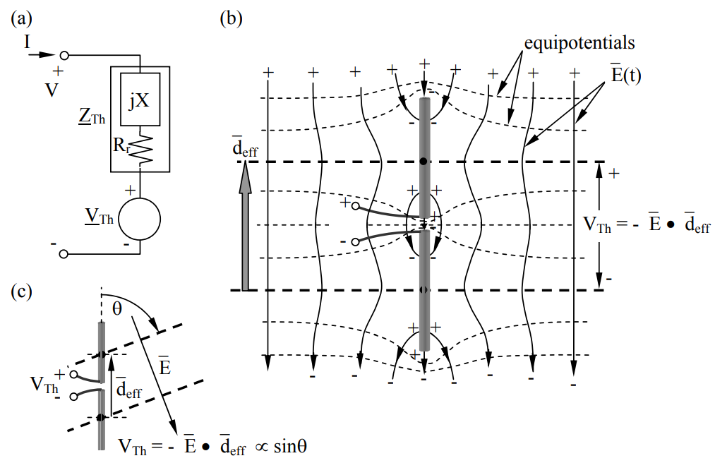
Far from the dipole the field lines \( \overline{\mathrm{E}}\) in Figure 10.3.1(b) are those of the quasistatic incident plane wave, i.e., uniform and parallel to the dipole. Close to the conducting dipole \( \overline{\mathrm{E}}\) is distorted to match the boundary conditions: 1) \( \overline{\mathrm{E}}_{||}\), and 2) each half of the dipole is an equipotential, intercepting only one equipotential line (boldface, dashed). If the wires comprising the short dipole are very thin, the effects of each wire on the other are negligible. Under these assumptions symmetry dictates the form for three of the equipotentials in Figure 10.3.1—the equipotentials through the center of the dipole and through each of its two halves are straight lines. The other equipotentials sketched with dashed lines curve around the conductors. The field lines \( \overline{\mathrm{E}}\) are sketched with solid lines locally perpendicular to the equipotentials. The field lines terminate at charges on the surface of the conductors and possibly at infinity, as governed by Gauss’s law: \(\hat{n} \bullet \overline{\mathrm{D}}=\sigma_{\mathrm{S}} \).

Figures 10.3.1(b) and (c) suggest why the open-circuit voltage V_Th of the short dipole antenna equals the potential difference between the centers of the two halves of this ideal dipole:

\[ \mathrm{V}_{\mathrm{Th}} \equiv-\overline{\mathrm{E}} \bullet \overline{\mathrm{d}}_{\mathrm{eff}} \qquad\qquad\qquad \text { (voltage induced on dipole antenna) }\]

The effective length of the dipole, \(\overline{\mathrm{d}}_{\mathrm{eff}} \), is defined by (10.3.19), and is the same as the effective length defined in terms of the current distribution (10.2.25) for infinitesimally thin straight wires of length d << λ. Generally \(\mathrm{d}_{\mathrm{eff}} \cong \mathrm{d} / 2 \), which is the distance between the centers of the two conductors. Each conductor is essentially sampling the electrostatic potential in its vicinity and conveying that to the antenna terminals. The orientation of \(\overline{\mathrm{d}}_{\mathrm{eff}} \) is that of the dipole current flow that would be driven by external sources having the defined terminal polarity.

The maximum power an antenna can deliver to an external circuit of impedance \( \underline{\mathrm{Z}}_{\mathrm{L}}\) is easily computed once the antenna equivalent circuit is known. To maximize this transfer it is first necessary to add an external load reactance, -jX_L, in series to cancel the antenna reactance +jX (X is negative for a short dipole antenna because it is capacitive). Then the resistive part of the load R_L must match that of the antenna, i.e., R_L = R_r. Maximum power transfer occurs when the impedances match so incident waves are not reflected. In this conjugate-match case (Z_L = Z_A*), the antenna Thevenin voltage \(\mathrm{\underline{V}_{T h}}\) is divided across the two resistors R_r and R_L so that the voltage across R_L is \(\mathrm{\underline{V}_{T h}} / 2\) and the power received by the short dipole antenna is:

\[\mathrm{P_{r}=\frac{1}{2 R_{r}}\left|\frac{\underline V_{T h}}{2}\right|^{2}} \ [W] \qquad\qquad\qquad(\text { received power })\]

Substitution into (10.3.20) of R_r (10.3.16) and V_Th (10.3.19) yields the received power:

\[\mathrm P_{\mathrm{r}}=\frac{3}{4 \eta_{0} \pi(\mathrm{d} / \lambda)^{2}}\left|\frac{\mathrm{\overline{\underline E}} \mathrm{d}_{\mathrm{eff}} \sin \theta}{2}\right|^{2}=\frac{|\overline{\mathrm{\underline E}}|^{2}}{2 \eta_{\mathrm{o}}} \frac{\lambda^{2}}{4 \pi}\left(1.5 \sin ^{2} \theta\right)\]

\[\mathrm P_{\mathrm{r}}=I(\theta, \varphi) \frac{\lambda^{2}}{4 \pi} \mathrm{G}(\theta, \varphi)=\mathrm{I}(\theta, \varphi) \mathrm{A}(\theta, \varphi) \ [\mathrm{W}] \qquad\qquad\qquad \text { (power received) }\]

where I(θ,φ) is the power intensity [Wm^-2] of the plane wave arriving from direction (θ,φ), G(θ,φ) = D(θ,φ) = 1.5 sin²θ is the antenna gain of a lossless short-dipole antenna (10.3.7), and A(θ,φ) is the antenna effective area as defined by the equation P_r ≡ I(θ,φ) A(θ,φ) [W] for the power received. Section 10.3.4 proves that the simple relation between gain G(θ,φ) and effective area A(θ,φ) proven in (10.3.22) for a short dipole applies to essentially all⁵³ antennas:

\[A(\theta, \varphi)=\frac{\lambda^{2}}{4 \pi} G(\theta, \varphi) \ \left[\mathrm m^{2}\right] \qquad\qquad\qquad \text { (antenna effective area) }\]

⁵³ This expression requires that all media near the antenna be reciprocal, which means that no magnetized plasmas or ferrites should be present so that the permittivity and permeabiliy matrices ε and μ everywhere equal their own transposes.

Equation (10.3.23) says that the effective area of a matched short-dipole antenna is equivalent to a square roughly λ/3 on a side, independent of antenna length. A small wire structure (<< λ/3) can capture energy from this much larger area if it has a conjugate match, which generally requires a high-Q resonance, large field strengths, and high losses. In practice, short-dipole antennas generally have a reactive mismatch that reduces their effective area below optimum.

Generalized relation between antenna gain and effective area

Section 10.3.3 proved for a short-dipole antenna the basic relation (10.3.23) between antenna gain G(θ,\(\phi\)) and antenna effective area A(θ,\(\phi\)):

\[\mathrm{A}(\theta, \phi)=\frac{\lambda^{2}}{4 \pi} \mathrm{G}(\theta, \phi)\]

This relation can be proven for any arbitrary antenna provided all media in and near the antenna are reciprocal media, i.e., their complex permittivity, permeability, and conductivity matrices \(\underline{\varepsilon}\), \(\underline{\mu}\), and \(\underline{\sigma}\) are all symmetric:

\[\underline{\varepsilon}=\underline{\varepsilon}^{\mathrm{t}}, \ \ \underline{\mu}=\underline{\mu}^{\mathrm{t}}, \ \ \underline{\sigma}=\underline{\sigma}^{\mathrm{t}}\]

where we define the transpose operator t such that \( \underline{\mathrm{A}}_{\mathrm{ij}}^{\mathrm{t}}=\underline{\mathrm{A}}_{\mathrm{ji}}\). Non-reciprocal media are rare, but include magnetized plasmas and magnetized ferrites; they are not discussed in this text. Media characterized by matrices are discussed in Section 9.5.1.

To prove (10.3.24) we characterize a general linear 2-port network by its impedance matrix:

\[\overline{\underline{\mathrm{Z}}}=\left[\begin{array}{ll} \underline{\mathrm{Z}}_{11} & \underline{\mathrm{Z}}_{12} \\ \underline{\mathrm{Z}}_{21} & \underline{\mathrm{Z}}_{22} \end{array}\right] \qquad\qquad\qquad \text{(impedance matrix)}\]

\[\overline{\mathrm{\underline V}}=\overline{\overline{\mathrm{\underline Z}}} \bar{\mathrm{\underline I}}\]

where \( \overline{\mathrm{\underline V}}\) and \( \overline{\mathrm{\underline I}}\) are the two-element voltage and current vectors \( \left[\mathrm{\underline{V}_{1}, \underline{V}_{2}}\right]\) and \(\left[\mathrm{\underline{I}_{1}, \underline{I}_{2}}\right] \), and \( \underline{\mathrm {V}}_{\mathrm i}\) and \( \underline{\mathrm {I}}_{\mathrm i}\) are the voltage and current at terminal pair i. This matrix \( \overline{\mathrm{\overline Z}}\) does not depend on the network to which the 2-port is connected. If the 2-port system is a reciprocal network, then \(\overline{\overline{\underline{\mathrm{Z}}}}=\overline{\overline{\underline{\mathrm{Z}}}}^{\mathrm t} \), so \(\underline{\mathrm{Z}}_{12}=\underline{\mathrm{Z}}_{21} \).

Since Maxwell’s equations are linear, \(\underline{\mathrm V} \) is linearly related to \( \underline{\mathrm I}\), and we can define an antenna impedance \( \underline{\mathrm Z}_{11}\) consisting of a real part (10.3.14), typically dominated by the radiation resistance Rr (10.3.12), and a reactive part jX (10.3.15). Thus \( \mathrm{\underline{Z}_{11}=R_{1}+j X_{1}}\), where R₁ equals the sum of the dissipative resistance R_d1 and the radiation resistance R_r1. For most antennas R_d << R_r.

Figure 10.3.2 illustrates an unknown reciprocal antenna (1) that communicates with a shortdipole test antenna (2) that is aimed at antenna (1). Because the relations between the voltages and currents at the terminals are determined by electromagnetic waves governed by the linear Maxwell equations, the two antennas constitute a two-port network governed by (10.3.26) and (10.3.27) and the complex impedance matrix \( \overline{\overline{\mathrm{\underline Z}}}\). Complex notation is appropriate here because antennas are frequency dependent. This impedance representation easily introduces the reciprocity constraint to the relation between G(θ,\(\phi\)) and A(θ,\(\phi\)). We assume each antenna is matched to its load \( \mathrm{\underline{Z}_{L}=R_{r}-j X}\) so as to maximize power transfer.

Figure \(\PageIndex{2}\): Coupled reciprocal antennas for relating G(θ,\(\phi\)) to A(θ,\(\phi\)).

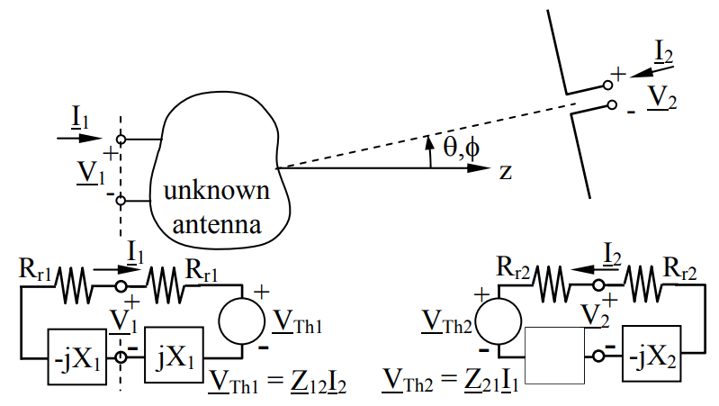
The power P_r received by each antenna and dissipated in the load can be expressed in two equivalent ways—in terms of antenna mutual impedance \(\underline{\mathrm Z}_{\mathrm{ij}} \) and in terms of antenna gain and effective area:

\[P_{\mathrm{r} 1}=\frac{\left|\mathrm{\underline V}_{\mathrm{Th} 1}\right|^{2}}{8 \mathrm{R}_{\mathrm{r} 1}}=\frac{\left|\mathrm{\underline Z}_{12} \mathrm{\underline I}_{2}\right|^{2}}{8 \mathrm{R}_{\mathrm{r} 1}}=\frac{\mathrm{G}_{2} \mathrm{P}_{\mathrm{t} 2}}{4 \pi \mathrm{r}^{2}} \mathrm{A}_{1}\]

\[P_{\mathrm{r} 2}=\frac{\left|\mathrm{\underline V}_{\mathrm{Th} 2}\right|^{2}}{8 \mathrm{R}_{\mathrm{r} 2}}=\frac{\left|\underline{\mathrm{Z}}_{21} \mathrm{\underline I}_{\mathrm{I}}\right|^{2}}{8 \mathrm{R}_{\mathrm{r} 2}}=\frac{\mathrm{G}_{1} \mathrm{P}_{\mathrm{t} 1}}{4 \pi \mathrm{r}^{2}} \mathrm{A}_{2}\]

Taking the ratio of these two equations in terms of G and A yields:

\[\frac{P_{r 2}}{P_{r 1}}=\frac{G_{1} A_{2} P_{t 1}}{G_{2} A_{1} P_{t 2}}\]

\[\therefore \frac{\mathrm{A}_{1}}{\mathrm{G}_{1}}=\frac{\mathrm{A}_{2}}{\mathrm{G}_{2}} \frac{\mathrm{P}_{\mathrm{t} 1} \mathrm{P}_{\mathrm{r} 1}}{\mathrm{P}_{\mathrm{t} 2} \mathrm{P}_{\mathrm{r} 2}}\]

But the ratio of the same equations in terms of \(\underline{\mathrm{Z}}_{\mathrm{ij}}\) also yields:

\[\mathrm{\frac{P_{\mathrm{r} 1}}{P_{\mathrm{r} 2}}=\frac{\left|\underline{Z}_{12} \underline I_{2}\right|^{2} R_{\mathrm{r} 2}}{\left|\underline Z_{21} \underline I_{1}\right|^{2}}=\frac{\left|\underline{Z}_{12}\right|^{2} P_{\mathrm{t} 2}}{\left|\underline Z_{2}\right|^{2} P_{\mathrm{t} 1}}}\]

Therefore if reciprocity applies, so that \( \mathrm{\left|\underline{Z}_{12}\right|^{2}=\left|\underline{Z}_{21}\right|^{2}}\), then (10.3.23) for a short dipole and substitution of (10.3.32) into (10.3.31) proves that all reciprocal antennas obey the same A/G relationship:

\[\frac{\mathrm{A}_{1}(\theta, \phi)}{\mathrm{G}_{1}(\theta, \phi)}=\frac{\mathrm{A}_{2}}{\mathrm{G}_{2}}=\frac{\lambda^{2}}{4 \pi} \qquad \qquad \qquad \text{(generalized gain-area relationship) }\]

Communication links

We now can combine the transmitting and receiving properties of antennas to yield the power that can be transmitted from one place to another. For example, the intensity I(θ,\(\phi\)) at distance r that results from transmitting P_t watts from an antenna with gain G_t(θ,\(\phi\)) is:

\[\mathrm{I}(\theta, \phi)=\mathrm{G}(\theta, \phi) \frac{\mathrm{P}_{\mathrm{t}}}{4 \pi \mathrm{r}^{2}} \ \left[\mathrm{W} / \mathrm{m}^{2}\right] \qquad \qquad \qquad \text{(radiated intensity)}\]

The power received by an antenna with effective area A(θ,\(\phi\)) in the direction θ,\(\phi\) from which the signal arrives is:

\[\mathrm{P}_{\mathrm{r}}=\mathrm{I}(\theta, \phi) \mathrm{A}(\theta, \phi) \ [\mathrm{W}] \qquad \qquad \qquad \text{(received power)}\]

where use of the same angles θ,\(\phi\) for the transmission and reception implies here that the same ray is being both transmitted and received, even though the transmitter and receiver coordinate systems are typically distinct. Equation (10.3.33) says:

\[\mathrm{A}(\theta, \phi)=\frac{\lambda^{2}}{4 \pi} \mathrm{G}_{\mathrm{r}}(\theta, \phi)\]

where G_r is the gain of the receiving antenna, so the power received (10.3.35) becomes:

\[\mathrm{P_{r}=\frac{P_{t}}{4 \pi r^{2}} G_{t}(\theta, \phi) \frac{\lambda^{2}}{4 \pi} G_{r}(\theta, \phi)=P_{t} G_{t}(\theta, \phi) G_{r}(\theta, \phi)\left(\frac{\lambda}{4 \pi r}\right)^{2} }\ [W]\]

Although (10.3.37) suggests the received power becomes infinite as r → 0, this would violate the far-field assumption that r >> λ/2\(\pi\).

Example \(\PageIndex{C}\)

Two wireless phones with matched short dipole antennas having d_eff equal one meter communicate with each other over a ten kilometer unobstructed path. What is the maximum power P_A available to the receiver if one watt is transmitted at f = 1 MHz? At 10 MHz? What is P_A at 1 MHz if the two dipoles are 45° to each other?

Solution

P_A = AI, where A is the effective area of the receiving dipole and I is the incident wave intensity [W m^-2]. \(\mathrm{P_{A}=A\left(P_{t} G_{t} / 4 \pi r^{2}\right)}\) where \(\mathrm{A=G_{r} \lambda^{2} / 4 \pi} \) and G_t ≤1.5; G_r ≤1.5. Thus \( \mathrm{P_{A}=\left(G_{r} \lambda^{2} / 4 \pi\right)\left(P_{t} G_{t} / 4 \pi r^{2}\right)=P_{t}(1.5 \lambda / 4 \pi r)^{2}=P_{t}(1.5 c / 4 \pi r f)^{2}}=1\left(1.5 \times 3 \times 10^{8} / 4 \pi 10^{4} \times 10^{6}\right)^{2} \cong 1.3 \times 10^{-5} \ [\mathrm{W}]\). At 10 MHz the available power out is ~1.3×10^-7 [W]. If the dipoles are 45° to each other, the receiving cross section is reduced by a factor of \(\sin ^{2} 45^{\circ}=0.5 \Rightarrow P_{\mathrm{A}} \cong 6.4 \times 10^{-6}\ [\mathrm{W}] \).

Example \(\PageIndex{D}\)

In terms of the incident electric field \( \underline{\mathrm{E}}_{0}\), what is the maximum Thevenin equivalent voltage source \( \mathrm{\underline{V}_{T h}}\) for a small N-turn loop antenna operating at frequency f? A loop antenna is made by winding N turns of a wire in a flat circle of diameter D, where D << λ. If N = 1, what must D be in order for this loop antenna to have the same maximum \( \mathrm{\underline{V}_{T h}}\) as a short dipole antenna with effective length d_eff?

Solution

The open-circuit voltage \( \mathrm{\underline{V}_{T h}}\) induced at the terminals of a small wire loop (D << λ) follows from Ampere’s law: \(\underline{\mathrm{V}}_{\mathrm{Th}}=\int_{\mathrm{C}} \overline{\mathrm{\underline E}} \bullet \mathrm{d} \overline{\mathrm{s}}=-\mathrm{N} \int \int \mathrm{j} \omega \mu_{\mathrm{o}} \overline{\mathrm{\underline H}} \bullet \mathrm{d} \overline{\mathrm{a}}=-\mathrm{Nj} \omega \mu_{\mathrm{o}} \underline{\mathrm{H}} \pi \mathrm{D}^{2} / 4=-\mathrm{Nj} \omega \mu_{\mathrm{o}} \mathrm{\underline E} \pi \mathrm{D}^{2} / 4 \eta_{\mathrm{o}} \). But \( \omega \mu_{\mathrm{o}} \pi / 4 \eta_{\mathrm{o}}=\mathrm{f} \pi^{2} / 2 \mathrm{c}\), so \( \left|\underline{\mathrm V}_{\mathrm{T h}}\right|=\mathrm{Nf} \pi^{2}\left|\mathrm{\underline E}_{\mathrm{o}}\right| \mathrm{D}^{2} / 2 \mathrm{c}\). For a short dipole antenna the maximum \(\left|\underline{\mathrm V}_{\mathrm{Th}}\right|=\mathrm{d}_{\mathrm{eff}}\left|\underline{\mathrm{E}}_{\mathrm{o}}\right| \), so \( \mathrm{D}=\left(2 \mathrm{cd}_{\mathrm{eff}} / \mathrm{f} \pi^{2} \mathrm{N}\right)^{0.5}=\left(2 \lambda \mathrm{d}_{\mathrm{eff}} / \pi^{2} \mathrm{N}\right)^{0.5} \cong 0.45\left(\mathrm{d}_{\mathrm{eff}} \lambda / \mathrm{N}\right)^{0.5}\).