13.3: Acoustic Radiation and Antennas

Any mechanically vibrating surface can radiate acoustic waves. As in the case of electromagnetic waves, it is easiest to understand a point source first, and then to superimpose such radiators in combinations that yield the total desired radiation pattern. Reciprocity applies to linear acoustics, so the receiving and transmitting properties of acoustic antennas are proportional, as they are for electromagnetic waves; i.e. \(G(θ,φ) ∝ A(θ,φ)\).

The acoustic wave equation for pressure permits analysis of an acoustic monopole radiator:

\[\left[\nabla^{2}+\left(\omega / \mathrm c_{\mathrm{s}}\right)^{2}\right] \mathrm{\underline p}=0 \label{13.3.1}\]

If the acoustic radiator is simply an isolated sphere with a sinusoidally oscillating radius \(\underline{\mathrm{a}} \), then the source is spherically symmetric and so is the solution; thus \(∂/∂θ = ∂/∂φ = 0\). If we define \(ω/c_s = k\), then (\ref{13.3.1}) becomes:

\[\left[\mathrm{r}^{-2} \mathrm{d}\left(\mathrm{r}^{2} \mathrm{d} / \mathrm{dr}\right)+\mathrm{k}^{2}\right] \mathrm{\underline p}=\left[\mathrm{d}^{2} / \mathrm{dr}^{2}+2 \mathrm{r}^{-1} \mathrm{d} / \mathrm{dr}+\mathrm{k}^{2}\right] \mathrm{\underline p}=0 \label{13.3.2}\]

This can be rewritten more simply as:

\[\mathrm{d}^{2}(\mathrm{r\underline p}) / \mathrm{dr}^{2}+\mathrm{k}^{2}(\mathrm{r \underline p})=0 \label{13.3.3}\]

This equation is satisfied if \(\mathrm{r\underline p}\) is an exponential, so a radial acoustic wave propagating outward would have the form:

\[\mathrm{\underline{p}(r)=\underline{K} r^{-1} e^{-j k r} \ \left[N \ m^{-2}\right]} \label{13.3.4}\]

The associated acoustic velocity \( \underline{\mathrm{\overline u}}(\mathrm{r})\) follows from the complex form of Newton’s law (13.1.7): \(\mathrm{\nabla \underline{p} \cong-j \omega \rho_{o} \overline{\underline{u}} \ \left[N \ m^{-3}\right]} \):

\[\underline{\mathrm{\overline u}}(\mathrm{r})=-\nabla \mathrm{\underline p} / \mathrm{j} \omega \mathrm{r}_{\mathrm{o}}=\hat{r} \underline{\mathrm{K}}\left(\eta_{\mathrm{s}} \mathrm{r}\right)^{-1}\left[1+(\mathrm{jkr})^{-1}\right] \mathrm{e}^{-\mathrm{jkr}} \label{13.3.5}\]

The first and second terms in the solution (\ref{13.3.5}) correspond to the acoustic far field and acoustic near field, respectively. When kr >> 1 or, equivalently, r >> λ/2\(\pi\), then the near field term can be neglected, so that the far-field velocity corresponding to (\ref{13.3.4}) is:

\[\underline{\mathrm{\overline u}}_{\mathrm{ff}}(\mathrm{r})=\hat{r} \underline{\mathrm{K}}\left(\eta_{\mathrm{s}} \mathrm{r}\right)^{-1} \mathrm{e}^{-\mathrm{j} \mathrm{kr}} \left[\mathrm{m} \ \mathrm{s}^{-1}\right] \qquad \qquad \qquad \text{(far-field acoustic velocity)} \label{13.3.6}\]

The near-field velocity from (\ref{13.3.5}) is:

\[\underline{\mathrm{\overline u}}_{\mathrm{nf}}=-\mathrm{j} \mathrm{\underline K} \hat{r}\left(\mathrm{k} \eta_{\mathrm{s}} \mathrm{r}^{2}\right)^{-1} \mathrm{e}^{-\mathrm{j} \mathrm{kr}} \ \left[\mathrm{m} \ \mathrm{s}^{-1}\right] \qquad \qquad \qquad \text{(near-field acoustic velocity) } \label{13.3.7}\]

Since k = ω/c_s, the near-field velocity is proportional to ω^-1, and becomes very large at low frequencies. Thus a velocity microphone, i.e., one that responds to acoustic velocity u rather than to pressure, will respond much more strongly to low frequencies than to high ones when the microphone is held close to one’s lips (r > λ/2\(\pi\)), although they are sensitive to local wind turbulence.

The acoustic intensity I(r) can be computed using (13.1.22) for a sphere of radius \(\underline{\mathrm{a}} \) oscillating with a surface velocity \(\underline{\mathrm{u}}_{\mathrm{o}} \) at r = a. In this case \(\underline{\mathrm{\overline u}}(\mathrm{a})=\hat{r} \underline{\mathrm{u}}_{\mathrm{o}} \), and substituting this value for \( \underline{\mathrm{\overline u}}\) into (\ref{13.3.7}) yields the constant \( \mathrm{\underline{K}=j \underline{u}_{0} \eta_{s} a^{2}}\); this near-field equation is appropriate only if a << λ/2\(\pi\). Thus, using (\ref{13.3.4}) and (\ref{13.3.6}), the far field intensity is:

\[\mathrm{I}=\mathrm{R}_{\mathrm{e}}\left\{\mathrm{\underline{pu}}^{*}\right\} / 2=\left\lfloor\left.\underline{\mathrm{K}}\right|^{2} / 2 \eta_{\mathrm{s}} \mathrm{r}^{2}=\eta_{\mathrm{s}}\left|2 \pi \underline{\mathrm{u}}_{0} \mathrm{a}^{2}\right|^{2} \Big/ 2 \ \left[\mathrm{W} \ \mathrm{m}^{-2}\right]\right. label{13.3.8}\]

Integrating I over a sphere of radius r yields the total acoustic power transmitted:

\[\mathrm{P}_{\mathrm{t}}=2 \pi \eta_{\mathrm{s}}\left|\omega \mathrm{a}^{2} \underline{\mathrm{u}}_{\mathrm{o}} / \mathrm{c}_{\mathrm{s}}\right|^{2 \ }[\mathrm{W}] \qquad \qquad \qquad \text{(acoustic power radiated) } \label{13.3.9}\]

where 2\(\pi\)/λ = ω/c_s has been substituted. Thus P_t is proportional to \( \eta_{\mathrm{s}} \omega^{2} \mathrm{a}^{4}\left(\mathrm{u}_{\mathrm{o}} / \mathrm{c}_{\mathrm{s}}\right)^{2}\). This suggests the importance of using a high frequency ω and large radius a if substantial power is to be radiated using a velocity source \(\underline{\mathrm{u}}_{\mathrm{o}} \).

If we imagine a Thevenin equivalent acoustic source providing a “current” of u_o, then, using (\ref{13.3.9}), the acoustic radiation resistance of this acoustic antenna is:

\[\mathrm{R}_{\mathrm{r}}=\mathrm{P}_{\mathrm{t}} \Big/\left(\left|\underline{\mathrm{u}}_{\mathrm{o}}\right|^{2} / 2\right)=4 \pi \eta_{\mathrm{s}}\left(\mathrm{ka}^{2}\right)^{2} \ \left[\mathrm{kg} \ \mathrm{s}^{-1}\right] \label{13.3.10}\]

Arrays of such acoustic sources can synthesis a wide variety of antenna patterns because superposition applies and thus acoustic pressure and velocities will tend to cancel in some directions and add in others. For example, two such equal sources spaced distance d along the z axis, close compared to a wavelength and driven out of phase, would radiate the far-field pressure:

\[\underline{\mathrm p}(\mathrm{r}) \cong\left(\mathrm j \mathrm{k} \eta_{\mathrm{s}} \mathrm{a}^{2} \underline{\mathrm{u}}_{\mathrm{o}} / \mathrm{r}\right)\left(\mathrm{e}^{-\mathrm{j} \mathrm{kr}_{1}}-\mathrm{e}^{-\mathrm{j} \mathrm{kr}_{2}}\right)=\left(2 \mathrm{k} \eta_{\mathrm{s}} \mathrm{a}^{2} \underline{\mathrm{u}}_{\mathrm{o}} / \mathrm{r}\right) \sin [(\mathrm{kd} / 2) \cos \theta] \mathrm{e}^{-\mathrm{j} \mathrm{kr}} \label{13.3.11}\]

where r_1,2 ≅ r ± (d/2)cosθ. In the limit where kd = 2\(\pi\)d/λ << 1, (\ref{13.3.11}) becomes:

\[\mathrm{p}(\mathrm{r}) \cong\left(\mathrm{k}^{2} \mathrm{d} \eta_{\mathrm{s}} \mathrm{a}^{2} \underline{\mathrm{u}}_{\mathrm{o}} / \mathrm{r}\right) \cos \theta \mathrm{e}^{-\mathrm{j} \mathrm{kr}} \label{13.2.12}\]

The radiated intensity I(θ) for this acoustic dipole is sketched in Figure 13.3.1(a), and is proportional to p² and therefore to k⁴ and ω⁴.

Figure \(\PageIndex{1}\): Acoustic radiators: (a) dipole, (b) loudspeaker, (c) baffled loudspeaker.

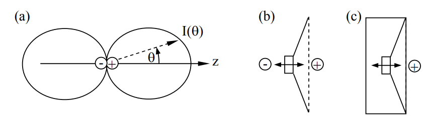
Thus it radiates poorly at low frequencies. Its acoustic antenna gain G(θ) is 3cos²θ, which can be computed by comparing the acoustic intensity I to the total acoustic power radiated P_t, just as is done for electromagnetic antennas. That is, the acoustic gain over an isotropic radiator is:

\[\mathrm{G}(\theta, \phi)=\mathrm{I}(\theta, \phi, \mathrm{r}) \big/\left[\mathrm{P}_{\mathrm{t}} / 4 \pi \mathrm{r}^{2}\right] \qquad \qquad \qquad \text{(acoustic antenna gain)} \label{13.3.13}\]

\[\mathrm{P_{t}=\int_{0}^{2 \pi \pi} \int_{0}^{I(\theta, \phi, r) r^{2}} \sin \theta \ d \theta \ d \phi \ [W]} \label{13.3.14}\]

A common way to produce this dipole acoustic pattern is illustrated in Figure 13.3.1(b) for the case of a loudspeaker with no baffling to block radiation from the back side of its vibrating speaker cone; the back side is clearly 180^o out of phase with the velocity of the front side. The radiation from an unbaffled loudspeaker can unfortunately reflect from the walls of the room and interfere with the sound from the front side, reinforcing those frequencies for which the two rays add in phase, and diminishing those frequencies for which they are out of phase. As a result, most good loudspeakers are baffled so the reverse wave is trapped and cannot interfere with the primary wave radiated forward. This alters the acoustic impedance of the loudspeaker, but it can be electrically compensated. The result is an acoustic monopole that radiates total power in proportion to p², k², and therefore ω², rather than ω⁴ as for the dipole.

A linear array of monopole acoustic sources of total length L has a diffraction pattern similar to that for an array of Hertzian dipoles. If the sources are all in phase, then they radiate maximum power broadside (θ ≡ 0) where all rays remain in phase. They exhibit their first null at θ ≅ ±λ/L. See Section 10.4 for more discussion of arrays of radiators. Acoustic array microphones have similar directional patterns, and microphones feeding parabolic reflectors of large dimension L have even higher gains, where the gain of an acoustic antenna is proportional to its effective area. The effective area of a parabolic reflector large compared to a wavelength is approximately its physical cross-section if it is uniformly illuminated without spillover, as shown in (11.1.25) for electromagnetic waves.