
3.5: Force on a Dipole in an Inhomogeneous Electric Field


- Last updated
- Mar 5, 2022
- Save as PDF

\newcommand{\vecs}[1]{\overset { \scriptstyle \rightharpoonup} {\mathbf{#1}} }
\newcommand{\vecd}[1]{\overset{-\!-\!\rightharpoonup}{\vphantom{a}\smash {#1}}}
\newcommand{\id}{\mathrm{id}} \newcommand{\Span}{\mathrm{span}}
( \newcommand{\kernel}{\mathrm{null}\,}\) \newcommand{\range}{\mathrm{range}\,}
\newcommand{\RealPart}{\mathrm{Re}} \newcommand{\ImaginaryPart}{\mathrm{Im}}
\newcommand{\Argument}{\mathrm{Arg}} \newcommand{\norm}[1]{\| #1 \|}
\newcommand{\inner}[2]{\langle #1, #2 \rangle}
\newcommand{\Span}{\mathrm{span}}
\newcommand{\id}{\mathrm{id}}
\newcommand{\Span}{\mathrm{span}}
\newcommand{\kernel}{\mathrm{null}\,}
\newcommand{\range}{\mathrm{range}\,}
\newcommand{\RealPart}{\mathrm{Re}}
\newcommand{\ImaginaryPart}{\mathrm{Im}}
\newcommand{\Argument}{\mathrm{Arg}}
\newcommand{\norm}[1]{\| #1 \|}
\newcommand{\inner}[2]{\langle #1, #2 \rangle}
\newcommand{\Span}{\mathrm{span}} \newcommand{\AA}{\unicode[.8,0]{x212B}}
\newcommand{\vectorA}[1]{\vec{#1}} % arrow
\newcommand{\vectorAt}[1]{\vec{\text{#1}}} % arrow
\newcommand{\vectorB}[1]{\overset { \scriptstyle \rightharpoonup} {\mathbf{#1}} }
\newcommand{\vectorC}[1]{\textbf{#1}}
\newcommand{\vectorD}[1]{\overrightarrow{#1}}
\newcommand{\vectorDt}[1]{\overrightarrow{\text{#1}}}
\newcommand{\vectE}[1]{\overset{-\!-\!\rightharpoonup}{\vphantom{a}\smash{\mathbf {#1}}}}
\newcommand{\vecs}[1]{\overset { \scriptstyle \rightharpoonup} {\mathbf{#1}} }
\newcommand{\vecd}[1]{\overset{-\!-\!\rightharpoonup}{\vphantom{a}\smash {#1}}}
\newcommand{\avec}{\mathbf a} \newcommand{\bvec}{\mathbf b} \newcommand{\cvec}{\mathbf c} \newcommand{\dvec}{\mathbf d} \newcommand{\dtil}{\widetilde{\mathbf d}} \newcommand{\evec}{\mathbf e} \newcommand{\fvec}{\mathbf f} \newcommand{\nvec}{\mathbf n} \newcommand{\pvec}{\mathbf p} \newcommand{\qvec}{\mathbf q} \newcommand{\svec}{\mathbf s} \newcommand{\tvec}{\mathbf t} \newcommand{\uvec}{\mathbf u} \newcommand{\vvec}{\mathbf v} \newcommand{\wvec}{\mathbf w} \newcommand{\xvec}{\mathbf x} \newcommand{\yvec}{\mathbf y} \newcommand{\zvec}{\mathbf z} \newcommand{\rvec}{\mathbf r} \newcommand{\mvec}{\mathbf m} \newcommand{\zerovec}{\mathbf 0} \newcommand{\onevec}{\mathbf 1} \newcommand{\real}{\mathbb R} \newcommand{\twovec}[2]{\left[\begin{array}{r}#1 \\ #2 \end{array}\right]} \newcommand{\ctwovec}[2]{\left[\begin{array}{c}#1 \\ #2 \end{array}\right]} \newcommand{\threevec}[3]{\left[\begin{array}{r}#1 \\ #2 \\ #3 \end{array}\right]} \newcommand{\cthreevec}[3]{\left[\begin{array}{c}#1 \\ #2 \\ #3 \end{array}\right]} \newcommand{\fourvec}[4]{\left[\begin{array}{r}#1 \\ #2 \\ #3 \\ #4 \end{array}\right]} \newcommand{\cfourvec}[4]{\left[\begin{array}{c}#1 \\ #2 \\ #3 \\ #4 \end{array}\right]} \newcommand{\fivevec}[5]{\left[\begin{array}{r}#1 \\ #2 \\ #3 \\ #4 \\ #5 \\ \end{array}\right]} \newcommand{\cfivevec}[5]{\left[\begin{array}{c}#1 \\ #2 \\ #3 \\ #4 \\ #5 \\ \end{array}\right]} \newcommand{\mattwo}[4]{\left[\begin{array}{rr}#1 \amp #2 \\ #3 \amp #4 \\ \end{array}\right]} \newcommand{\laspan}[1]{\text{Span}\{#1\}} \newcommand{\bcal}{\cal B} \newcommand{\ccal}{\cal C} \newcommand{\scal}{\cal S} \newcommand{\wcal}{\cal W} \newcommand{\ecal}{\cal E} \newcommand{\coords}[2]{\left\{#1\right\}_{#2}} \newcommand{\gray}[1]{\color{gray}{#1}} \newcommand{\lgray}[1]{\color{lightgray}{#1}} \newcommand{\rank}{\operatorname{rank}} \newcommand{\row}{\text{Row}} \newcommand{\col}{\text{Col}} \renewcommand{\row}{\text{Row}} \newcommand{\nul}{\text{Nul}} \newcommand{\var}{\text{Var}} \newcommand{\corr}{\text{corr}} \newcommand{\len}[1]{\left|#1\right|} \newcommand{\bbar}{\overline{\bvec}} \newcommand{\bhat}{\widehat{\bvec}} \newcommand{\bperp}{\bvec^\perp} \newcommand{\xhat}{\widehat{\xvec}} \newcommand{\vhat}{\widehat{\vvec}} \newcommand{\uhat}{\widehat{\uvec}} \newcommand{\what}{\widehat{\wvec}} \newcommand{\Sighat}{\widehat{\Sigma}} \newcommand{\lt}{<} \newcommand{\gt}{>} \newcommand{\amp}{&} \definecolor{fillinmathshade}{gray}{0.9}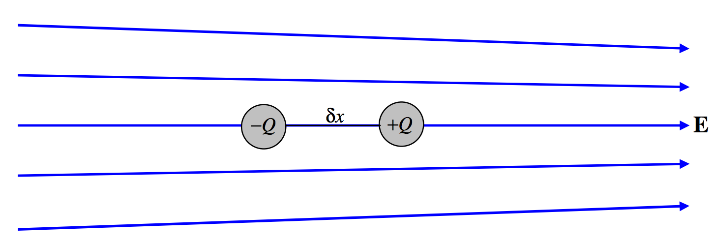 \text{FIGURE III.4}
Consider a simple dipole consisting of two charges +Q and -Q separated by a distance δx, so that its dipole moment is p = Q\, δx. Imagine that it is situated in an inhomogeneous electrical field as shown in Figure III.4. We have already noted that a dipole in a homogeneous field experiences no net force, but we can see that it does experience a net force in an inhomogeneous field. Let the field at −Q \text{ be }E and the field at +Q \text{ be }E + δE. The force on −Q \text{ is }QE to the left, and the force on +Q \text{ is }Q(E + δE) to the right. Thus there is a net force to the right of Q\, δE, or:
\label{3.5.1}\text{Force}=p\frac{dE}{dx}
Equation \ref{3.5.1} describes the situation where the dipole, the electric field and the gradient are all parallel to the x-axis. In a more general situation, all three of these are in different directions. Recall that electric field is minus potential gradient. Potential is a scalar function, whereas electric field is a vector function with three component, of which the x-component, for example is E_x=-\frac{∂V}{∂x}. Field gradient is a symmetric tensor having nine components (of which, however, only six are distinct), such as \frac{∂^2V}{ ∂x^2},\,\frac{ ∂^2V}{ ∂y ∂z} etc. Thus in general Equation \ref{3.5.1} would have to be written as
\begin{pmatrix}E_x \\ E_y \\ E_z \\ \end{pmatrix} =-\begin{pmatrix}V_{xx} & V_{xy} & V_{xz} \\ V_{xy} & V_{yy} & V_{yz} \\ V_{xz} & V_{yz} & V_{zz} \\ \end{pmatrix}\begin{pmatrix}p_x \\ p_y \\ p_z \\ \end{pmatrix}\label{3.5.2}
in which the double subscripts in the potential gradient tensor denote the second partial derivatives.