10.2: Electromagnetic Induction and the Lorentz Force

Last updated
Save as PDF

Page ID: 5474

\( \newcommand{\vecs}[1]{\overset { \scriptstyle \rightharpoonup} {\mathbf{#1}} } \) \( \newcommand{\vecd}[1]{\overset{-\!-\!\rightharpoonup}{\vphantom{a}\smash {#1}}} \)\(\newcommand{\id}{\mathrm{id}}\) \( \newcommand{\Span}{\mathrm{span}}\) \( \newcommand{\kernel}{\mathrm{null}\,}\) \( \newcommand{\range}{\mathrm{range}\,}\) \( \newcommand{\RealPart}{\mathrm{Re}}\) \( \newcommand{\ImaginaryPart}{\mathrm{Im}}\) \( \newcommand{\Argument}{\mathrm{Arg}}\) \( \newcommand{\norm}[1]{\| #1 \|}\) \( \newcommand{\inner}[2]{\langle #1, #2 \rangle}\) \( \newcommand{\Span}{\mathrm{span}}\) \(\newcommand{\id}{\mathrm{id}}\) \( \newcommand{\Span}{\mathrm{span}}\) \( \newcommand{\kernel}{\mathrm{null}\,}\) \( \newcommand{\range}{\mathrm{range}\,}\) \( \newcommand{\RealPart}{\mathrm{Re}}\) \( \newcommand{\ImaginaryPart}{\mathrm{Im}}\) \( \newcommand{\Argument}{\mathrm{Arg}}\) \( \newcommand{\norm}[1]{\| #1 \|}\) \( \newcommand{\inner}[2]{\langle #1, #2 \rangle}\) \( \newcommand{\Span}{\mathrm{span}}\)\(\newcommand{\AA}{\unicode[.8,0]{x212B}}\)

Imagine that there is a uniform magnetic field directed into the plane of the paper (or your computer screen), as in Figure X.1. Suppose there is a metal rod, as in the Figure, and that the rod is being moved steadily to the right. We know that, within the metal, there are many free conduction electrons, not attached to any particular atom, but free to wander about inside the metal. As the metal rod is moved to the right, these free conduction electrons are also moving to the right and therefore they experience a Lorentz \(q\textbf{v}\times \textbf{B}\) force, which moves them down (remember – electrons are negatively charged) towards the bottom end of the rod. Thus the movement of the rod through the magnetic field induces a potential difference across the ends of the rod. We have achieved electromagnetic induction, and, seen this way, there is nothing new: electromagnetic induction is nothing more than the Lorentz force on the conduction electrons within the metal.

X.1.png

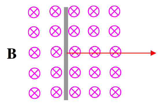
\(\text{FIGURE X.1}\)

You may speculate that, as an aircraft flies through Earth's magnetic field, a potential difference will be induced across the wingtips. You might try to imagine how you might set up an experiment to detect or measure this. You might also speculate that, as seawater flows up the English Channel, a potential difference is induced between England and France. You might also ask yourself: What if the rod were stationary, and the magnetic field were moving to the left? That's an interesting discussion for lunchtime: Can you imagine the magnetic field moving to the left? Who's to say whether the rod or the field is moving?

If we were somehow to connect the ends of the rod in Figure X.1 to a closed circuit, we might cause a current to flow – and we would then have made an electric generator. Look at Figure X.2.

X.2.png

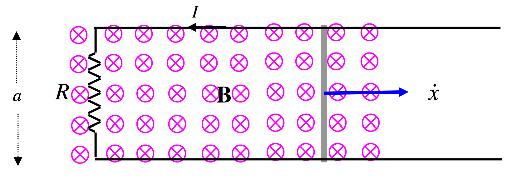
\(\text{FIGURE X.2}\)

We imagine that our metal bar is being pulled steadily to the right at speed \(v\), and that it is in contact with, and sliding smoothly without friction upon, two rails a distance \(a\) apart, and that the rails are connected via a resistance \(R\). As a consequence, a current \(I\) flows in the circuit in the direction shown, counterclockwise. (The current is, of course, made up of negative conduction electrons moving clockwise.) Now the magnetic field will exert a force on the current in the rod. The force on the rod will be a \(\textbf{I}\times\textbf{B}\); that is \(aIB\) acting to the left. In order to keep the rod moving steadily at speed \(v\) to the right against this force, work will have to be done at a rate \(aIBv\). The work will be dissipated in the resistance at a rate \(I\, V\) where \(V\) is the induced EMF. Therefore the induced EMF is \(Bav\). But \(av\) is the rate at which the area of the circuit is increasing, and \(Bav\) is the rate at which the magnetic \(B\)-flux through the circuit is increasing. Therefore the induced EMF is equal to the rate of change of magnetic flux through the circuit. Thus we have predicted Faraday's law quantitatively merely from what we already know about the forces on currents and charged particles in a magnetic field.