
1.1: The Coulomb Law


- Last updated
- Mar 5, 2022
- Save as PDF

( \newcommand{\kernel}{\mathrm{null}\,}\)
A quantitative discussion of classical electrodynamics, starting from the electrostatics, requires a common agreement on the meaning of the following notions:2
- electric charges qk, as revealed, most explicitly, by observation of electrostatic interaction between the charged particles;
- point charges – the charged particles so small that their position in space, for the given problem, may be completely described (in a given reference frame) by their radius-vectors rk; and
- electric charge conservation – the fact that the algebraic sum of all charges qk inside any closed volume is conserved unless the charged particles cross the volume’s border.
I will assume that these notions are well known to the reader. Using them, the Coulomb law3 for the interaction of two stationary point charges may be formulated as follows:
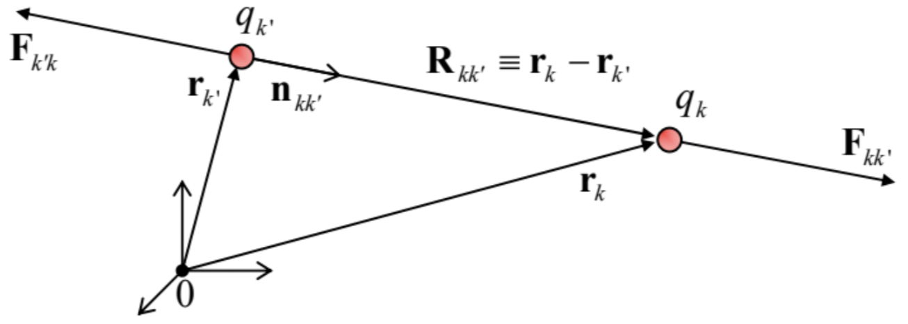
Coulomb LawFkk′=κqkqk′rk−rk′|rk−rk′|3≡κqkqk′R2kk′nkk′, with Rkk′≡rk−rk′,nkk′≡Rkk′Rkk′,Rkk′≡|Rkk′|.
where Fkk′ denotes the electrostatic (Coulomb) force exerted on the charge number k by the charge number k′, separated from it by distance Rkk′ – see Fig. 1.
I am confident that this law is very familiar to the reader, but a few comments may still be due:
- Flipping the indices k and k′, we see that Eq. (1) complies with the 3rd Newton law: the reciprocal force is equal in magnitude but opposite in direction: Fk′k=−Fkk′.
- Since the vector Rkk′≡rk−rk′, by its definition, is directed from the point rk′ toward the point rk (Fig. 1), Eq. (1) correctly describes the experimental fact that charges of the same sign (i.e. with qkqk′>0) repulse, while those with opposite signs (qkqk′<0) attract each other.
- In some textbooks, the Coulomb law (1) is given with the qualifier “in free space” or “in vacuum”. However, actually, Eq. (1) remains valid even in the presence of any other charges – for example, of internal charges in a quasi-continuous medium that may surround the two charges (number k and k′) under consideration. The confusion stems from the fact (to be discussed in detail in Chapter 3 below) that in some cases it is convenient to formally represent the effect of the other charges as an effective modification of the Coulomb law.
- The constant k in Eq. (1) depends on the system of units we use. In the Gaussian units, k is set to 1, for the price of introducing a special unit of charge (the statcoulomb) that would make experimental data compatible with Eq. (1), if the force Fkk′ is measured in the Gaussian units (dynes). On the other hand, in the International System (“SI”) of units, the charge’s unit is one coulomb (abbreviated C),4 and k is different from 1:
k|SI=14πε0,k in SI units
where ε0≈8.854×10⁻¹² is called the electric constant.
Unfortunately, the continuing struggle between zealous proponents of these two systems bears all not-so-nice features of a religious war, with a similarly slim chance for any side to win it in any foreseeable future. In my humble view, each of these systems has its advantages and handicaps (to be noted below on several occasions), and every educated physicist should have no problem with using any of them. Following insisting recommendations of international scientific unions, I am using the SI units through my series. However, for the readers’ convenience, in this course (where the difference between the Gaussian and SI systems is especially significant) I will write the most important formulas with the constant (2) clearly displayed – for example, Eq. (1) as
Fkk′=14πε0qkqk′rk−rk′|rk−rk′|3,
so that the transfer to the Gaussian units may be performed just by the formal replacement 4πε0→1. (In the rare cases when the transfer is not obvious, I will duplicate such formulas in the Gaussian units.)
Besides Eq. (3), another key experimental law of electrostatics is the linear superposition principle: the electrostatic forces exerted on some point charge (say, qk) by other charges add up as vectors, forming the net force
Fk=∑k′≠kFkk′,
where the summation is extended over all charges but qk, and the partial force Fkk′ is described by Eq. (3). The fact that the sum is restricted to k′≠k means that a point charge, in statics, does not interact with itself. This fact may look obvious from Eq. (3), whose right-hand side diverges at rk→rk′, but becomes less evident (though still true) in quantum mechanics – where the charge of even an elementary particle is effectively spread around some volume, together with particle’s wavefunction.5
Now we may combine Eqs. (3) and (4) to get the following expression for the net force F acting on a probe charge q located at point r:
F(r)=q14πε0∑rk′≠rqk′r−rk′|r−rk′|3.
This equality implies that it makes sense to introduce the notion of the electric field at point r (as an entity independent of q), characterized by the following vector:
Electric field: definitionE(r)≡F(r)q,
formally called the electric field strength – but much more frequently, just the “electric field”. In these terms, Eq. (5) becomes
Electric field of point chargesE(r)=14πε0∑rk′≠rqk′r−rk′|r−rk′|3.
Just convenient is electrostatics, the notion of the field becomes virtually unavoidable for the description of time-dependent phenomena (such as electromagnetic waves, see Chapter 7 and on), where the electromagnetic field shows up as a specific form of matter, with zero rest mass, and hence different from the usual “material” particles.
Many real-world problems involve multiple point charges located so closely that it is possible to approximate them with a continuous charge distribution. Indeed, let us consider a group of many (dN>>1) close charges, located at points rk′, all within an elementary volume d3r′. For relatively distant field observation points, with |r−rk′|≫dr′, the geometrical factor in the corresponding terms of Eq. (7) is
essentially the same. As a result, these charges may be treated as a single elementary charge dQ(r′). Since at dN≫1, this elementary charge is proportional to the elementary volume d3r′, we can define the local 3D charge density ρ(r′) by the following relation:
ρ(r′)d3r′≡dQ(r′)≡∑rk′∈d3r′qk′,
and rewrite Eq. (7) as an integral (over the volume containing all essential charges):
Electric field of continuous chargeE(r)=14πε0∫ρ(r′)r−r′|r−r′|3d3r′.
Note that for a continuous, smooth charge density ρ(r′), the integral in Eq. (9) does not diverge at R≡r−r′→ 0, because in this limit the fraction under the integral increases as R−2, i.e. slower than the decrease of the elementary volume d3r′, proportional to R3.
Let me emphasize the dual use of Eq. (9). In the case when ρ(r) is a continuous function representing the average charge, defined by Eq. (8), Eq. (9) is not valid at distances |r−rk′| of the order of the distance between the adjacent point charges, i.e. does not describe rapid variations of the electric field at these distances. Such approximate, smoothly changing field E(r), is called macroscopic; we will repeatedly return to this notion in the following chapters. On the other hand, Eq. (9) may be also used for the description of the exact (frequently called microscopic) field of discrete point charges, by employing the notion of Dirac’s δ-function, which is the mathematical approximation for a very sharp function equal to zero everywhere but one point, and still having a finite integral (equal to 1).6 Indeed, in this formalism, a set of point charges qk′ located in points rk′, may be represented by pseudo-continuous
density
ρ(r′)=∑k′qk′δ(r′−rk′).
Plugging this expression into Eq. (9), we return to its exact, discrete version (7). In this sense, Eq. (9) is
exact, and we may use it as the general expression for the electric field.
Reference
2 On top of the more general notions of the classical Newtonian space, point particles and forces, as used in classical mechanics – see, e.g., CM Sec. 1.1.
3 Formulated in 1785 by Charles-Augustin de Coulomb, on basis of his earlier experiments, in turn rooting in previous studies of electrostatic phenomena, with notable contributions by William Gilbert, Otto von Guericke, Charles François de Cisternay Du Fay, and Benjamin Franklin.
4 Since 2018, one coulomb is defined, in the “legal” metrology, as a certain, exactly fixed number of the fundamental electric charges e, and the “legal” SI value of E0 is not more exactly equal to 107/4πc2 (where c is the speed of light) as it was before that, but remains extremely close to that fraction, with the relative difference of the
order of 10−10 – see appendix CA: Selected Physical Constants.
5 Note that some widely used approximations, e.g., the density functional theory (DFT) of multi-particle systems, essentially violate this law, thus limiting their accuracy and applicability – see, e.g., QM Sec. 8.4.
6 See, e.g., MA Sec. 14. The 2D (areal) charge density σ and the 1D (linear) density λ may be defined absolutely similarly to the 3D (volumic) density ρ: dQ=σd2r,dQ=λdr. Note that the approximations in that either σ≠0 or λ≠0 imply that ρ is formally infinite at the charge location; for example, the model in that a plane z=0 is charged with areal density σ≠0, means that ρ=σδ(z), where δ(z) is Dirac’s delta function.