1.2: The Gauss Law

Due to the extension of Eq. (9) to point (“discrete”) charges, it may seem that we do not need anything else for solving any problem of electrostatics. In practice, however, this is not quite true – first of all, because the direct use of Eq. (9) frequently leads to complex calculations. Indeed, let us try to solve a very simple problem: finding the electric field induced by a spherically-symmetric charge distribution with density \(\ \rho\left(r^{\prime}\right)\). We may immediately use the problem’s symmetry to argue that the
electric field should be also spherically-symmetric, with only one component in the spherical coordinates: \(\ \mathbf{E}(\mathbf{r})=E(r) \mathbf{n}_{r}\), where \(\ \mathbf{n}_{r} \equiv \mathbf{r} / r\) is the unit vector in the direction of the field observation point \(\ \mathbf{r}\) (Fig. 2).

Fig. 1.2. One of the simplest problems of electrostatics: the electric field produced by a spherically-symmetric charge distribution.

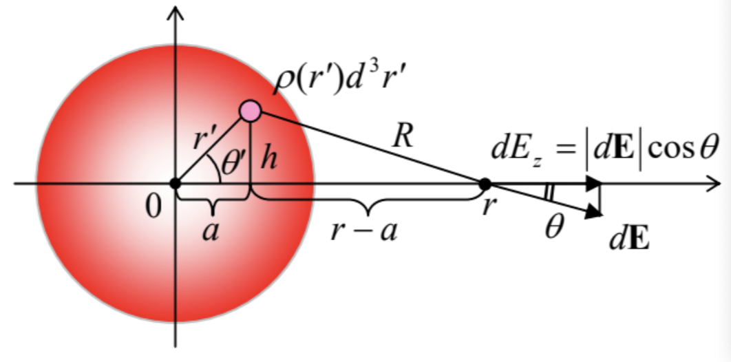
Taking this direction for the polar axis of a spherical coordinate system, we can use the evident axial symmetry of the system to reduce Eq. (9) to

\[\ E=\frac{1}{4 \pi \varepsilon_{0}} 2 \pi \int_{0}^{\pi} \sin \theta^{\prime} d \theta^{\prime} \int_{0}^{\infty} r^{\prime 2} d r^{\prime} \frac{\rho\left(r^{\prime}\right)}{R^{2}} \cos \theta,\tag{1.11}\]

where \(\ \theta\) and \(\ R\) are the geometrical parameters marked in Fig. 2. Since they all may be readily expressed via \(\ r^{\prime}\) and \(\ \theta^{\prime}\), using the auxiliary parameters \(\ a\) and \(\ h\),

\[\ \cos \theta=\frac{r-a}{R}, \quad R^{2}=h^{2}+\left(r-r^{\prime} \cos \theta\right)^{2}, \quad \text { where } a \equiv r^{\prime} \cos \theta^{\prime}, \quad h \equiv r^{\prime} \sin \theta^{\prime},\tag{1.12}\]

Eq. (11) may be eventually reduced to an explicit integral over \(\ r^{\prime}\) and \(\ \theta^{\prime}\), and worked out analytically, but that would require some effort.

For other problems, the integral (9) may be much more complicated, defying an analytical solution. One could argue that with the present-day abundance of computers and numerical algorithm libraries, one can always resort to numerical integration. This argument may be enhanced by the fact that numerical integration is based on the replacement of the required integral by a discrete sum, and the summation is much more robust to the (unavoidable) rounding errors than the finite-difference schemes typical for the numerical solution of differential equations. These arguments, however, are only partly justified, since in many cases the numerical approach runs into a problem sometimes called the curse of dimensionality – the exponential dependence of the number of needed calculations on the number of independent parameters of the problem.⁷ Thus, despite the proliferation of numerical methods in physics, analytical results have an everlasting value, and we should try to get them whenever we can. For our current problem of finding the electric field generated by a fixed set of electric charges, large help may come from the so-called Gauss law.

To derive it, let us consider a single point charge \(\ q\) inside a smooth, closed surface S (Fig. 3), and calculate product \(\ E_{n} d^{2} r\), where \(\ d^{2} r\) is an elementary area of the surface (which may be well approximated with a plane fragment of that area), and \(\ E_{n} \equiv \mathbf{E} \cdot \mathbf{n}\) is the component of the electric field at that point, normal to the plane.

Fig. 1.3. Deriving the Gauss law: a point charge \(\ q\) (a) inside the volume \(\ V\), and (b) outside of that volume.

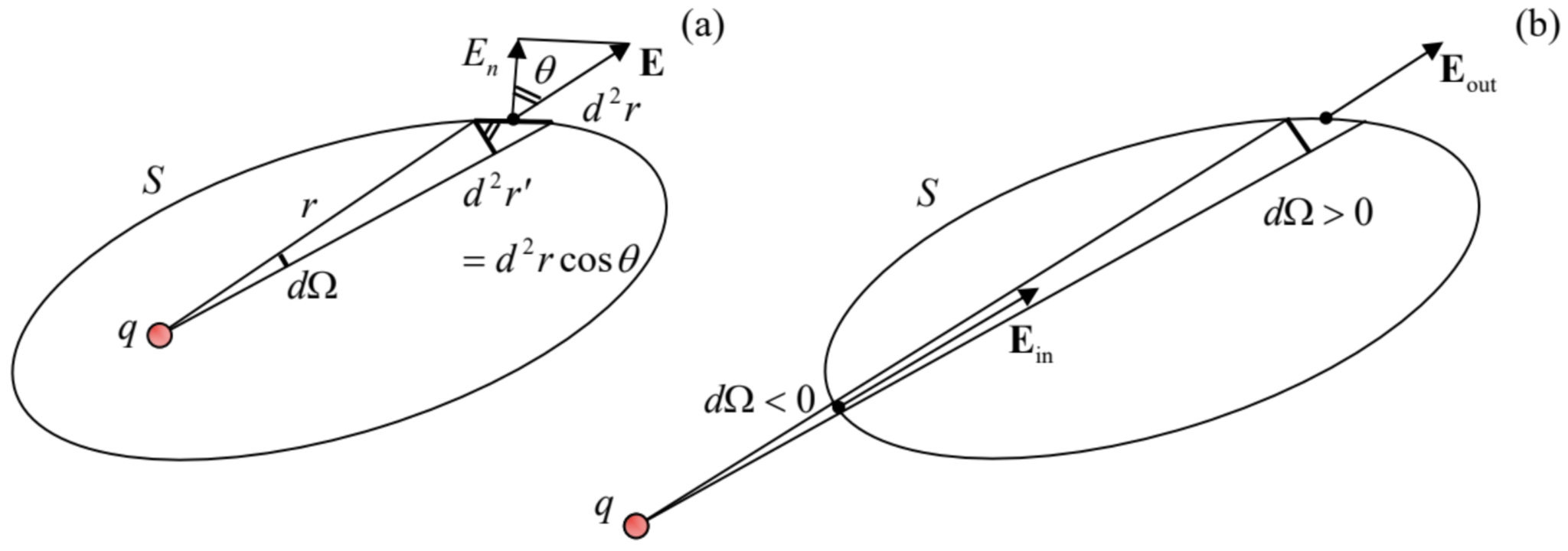
This component may be calculated as \(\ E \cos \theta\), where \(\ \theta\) is the angle between the vector E and the unit vector n normal to the surface. Now let us notice that the product \(\ \cos \theta d^{2} r\) is nothing more than the area \(\ d^{2}r^{\prime}\) of the projection of \(\ d^{2} r\) onto the plane perpendicular to vector r connecting the charge \(\ q\) with this point of the surface (Fig. 3), because the angle between the planes \(\ d^{2}r^{\prime}\) and \(\ d^{2} r\) is also equal to \(\ \theta\). Using the Coulomb law for E, we get

\[\ E_{n} d^{2} r=E \cos \theta d^{2} r=\frac{1}{4 \pi \varepsilon_{0}} \frac{q}{r^{2}} d^{2} r^{\prime}.\tag{1.13}\]

But the ratio \(\ d^{2} r^{\prime} / r^{2}\) is nothing more than the elementary solid angle \(\ d \Omega\) under which the areas \(\ d^{2}r^{\prime}\) and \(\ d^{2} r\) are seen from the charge point, so that \(\ E_{n} d^{2} r\) may be represented as just a product of \(\ d \Omega\) by a constant \(\ \left(q / 4 \pi \varepsilon_{0}\right)\). Summing these products over the whole surface, we get

\[\ \oint_{S} E_{n} d^{2} r=\frac{q}{4 \pi \varepsilon_{0}} \oint_{S} d \Omega \equiv \frac{q}{\varepsilon_{0}},\tag{1.14}\]

since the full solid angle equals \(\ 4 \pi\). (The integral on the left-hand side of this relation is called the flux of electric field through surface S.)

The relation (14) expresses the Gauss law for one point charge. However, it is only valid if the charge is located inside the volume \(\ V\) limited by the surface \(\ S\). To find the flux created by a charge located outside of the volume, we still can use Eq. (13), but have to be careful with the signs of the elementary contributions \(\ E_{n} d A\). Let us use the common convention to direct the unit vector n out of the closed volume we are considering (the so-called outer normal), so that the elementary product \(\ E_nd^2r=(\mathbf{E} \cdot \mathbf{n}) d^{2} r\) and hence \(\ d \Omega=E_{n} d^{2} r^{\prime} / r^{2}\) is positive if the vector E is pointing out of the volume (like in the example shown in Fig. 3a and the upper-right area in Fig. 3b), and negative in the opposite case (for example, in the lower-left area in Fig. 3b). As the latter figure shows, if the charge is located outside of the volume, for each positive contribution \(\ d \Omega\) there is always an equal and opposite contribution to the integral. As a result, at the integration over the solid angle, the positive and negative contributions cancel exactly, so that

\[\ \oint_{S} E_{n} d^{2} r=0.\tag{1.15}\]

The real power of the Gauss law is revealed by its generalization to the case of several charges within volume \(\ V\). Since the calculation of flux is a linear operation, the linear superposition principle (4) means that the flux created by several charges is equal to the (algebraic) sum of individual fluxes from each charge, for which either Eq. (14) or Eq. (15) are valid, depending on the charge position (in or out of the volume). As the result, for the total flux we get:

\[\ \oint_{S} E_{n} d^{2} r=\frac{Q_{V}}{\varepsilon_{0}} \equiv \frac{1}{\varepsilon_{0}} \sum_{\mathbf{r}_{j} \in V} q_{j} \equiv \frac{1}{\varepsilon_{0}} \int_{V} \rho\left(\mathbf{r}^{\prime}\right) d^{3} r^{\prime},\quad\quad\quad\text{Gauss Law}\tag{1.16}\]

where \(\ Q_{V}\) is the net charge inside volume \(\ V\). This is the full version of the Gauss law.⁸

In order to appreciate the problem-solving power of the law, let us return to the problem illustrated by Fig. 2, i.e. a spherical charge distribution. Due to its symmetry, which had already been discussed above, if we apply Eq. (16) to a sphere of radius r, the electric field should be normal to the sphere at each its point (i.e., \(\ E_{n}=E\)), and its magnitude the same at all points: \(\ E_{n}=E(r)\). As a result, the flux calculation is elementary:

\[\ \oint E_{n} d^{2} r=4 \pi r^{2} E(r)\tag{1.17}\]

Now, applying the Gauss law (16), we get:

\[\ 4 \pi r^{2} E(r)=\frac{1}{\varepsilon_{0}} \int_{r^{\prime}<r} \rho\left(r^{\prime}\right) d^{3} r^{\prime}=\frac{4 \pi}{\varepsilon_{0}} \int_{0}^{r} r^{\prime 2} \rho\left(r^{\prime}\right) d r^{\prime},\tag{1.18}\]

so that, finally,

\[\ E(r)=\frac{1}{r^{2} \varepsilon_{0}} \int_{0}^{r} r^{\prime 2} \rho\left(r^{\prime}\right) d r^{\prime}=\frac{1}{4 \pi \varepsilon_{0}} \frac{Q(r)}{r^{2}},\tag{1.19}\]

where \(\ Q(r)\) is the full charge inside the sphere of radius \(\ r\):

\[\ Q(r) \equiv \int_{r^{\prime}<r} \rho\left(r^{\prime}\right) d^{3} r^{\prime}=4 \pi \int_{0}^{r} \rho\left(r^{\prime}\right) r^{\prime 2} d r^{\prime}.\tag{1.20}\]

In particular, this formula shows that the field outside of a sphere of a finite radius \(\ R\) is exactly the same as if all its charge \(\ Q=Q(R)\) was concentrated in the sphere’s center. (Note that this important result is only valid for a spherically-symmetric charge distribution.) For the field inside the sphere, finding the electric field still requires the explicit integration (20), but this 1D integral is much simpler than the 2D integral (11), and in some important cases may be readily worked out analytically. For example, if the charge \(\ Q\) is uniformly distributed inside a sphere of radius \(\ R\),

\[\ \rho\left(r^{\prime}\right)=\rho=\frac{Q}{V}=\frac{Q}{(4 \pi / 3) R^{3}},\tag{1.21}\]

the integration is elementary:

\[\ E(r)=\frac{\rho}{r^{2} \varepsilon_{0}} \int_{0}^{r} r^{\prime 2} d r^{\prime}=\frac{\rho r}{3 \varepsilon_{0}}=\frac{1}{4 \pi \varepsilon_{0}} \frac{Q r}{R^{3}}.\tag{1.22}\]

We see that in this case, the field is growing linearly from the center to the sphere’s surface, and only at \(\ r>R\) starts to decrease in agreement with Eq. (19) with constant \(\ Q(r)=Q\). Note also that the electric field is continuous for all \(\ r\) (including \(\ r = R\)) – as for all systems with finite volumic density,

In order to underline the importance of the last condition, let us consider one more elementary but very important example of the Gauss law’s application. Let a thin plane sheet (Fig. 4) be charged uniformly, with an areal density \(\ \sigma=\operatorname{const}\). In this case, it is fruitful to use the Gauss volume in the form of a planar “pillbox” of thickness \(\ 2z\) (where \(\ z\) is the Cartesian coordinate perpendicular to the plane) and certain area \(\ A\) – see the dashed lines in Fig. 4. Due to the symmetry of the problem, it is evident that the electric field should be: (i) directed along the \(\ z\)-axis, (ii) constant on each of the upper and bottom sides of the pillbox, (iii) equal and opposite on these sides, and (iv) parallel to the side surfaces of the box. As a result, the full electric field flux through the pillbox’ surface is just \(\ 2 A E(z)\), so that the Gauss law (16) yields \(\ 2 A E(z)=Q_{A} / \varepsilon_{0} \equiv \sigma A / \varepsilon_{0}\), and we get a very simple but important formula

\[\ E(z)=\frac{\sigma}{2 \varepsilon_{0}}=\text { const }.\tag{1.23}\]

Fig. 1.4. The electric field of a charged plane.

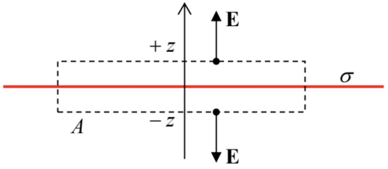
Notice that, somewhat counter-intuitively, the field magnitude does not depend on the distance from the charged plane. From the point of view of the Coulomb law (5), this result may be explained as follows: the farther the observation point from the plane, the weaker the effect of each elementary charge, \(\ d Q=\sigma d^{2} r\), but the more such elementary charges give contributions to the \(\ z\)-component of vector E, because they are “seen” from the observation point at relatively small angles to the \(\ z\)-axis.

Note also that though the magnitude \(\ E \equiv|\mathbf{E}|\) of the electric field is constant, its component \(\ E_{n}\) normal to the plane (for our coordinate choice, \(\ E_{z}\)) changes its sign at the plane, experiencing a discontinuity (jump) equal to

\[\ \Delta E_{n}=\frac{\sigma}{\varepsilon_{0}}.\tag{1.24}\]

This jump disappears if the surface is not charged. Returning for a split second to our charged sphere problem, solving it we considered the volumic charge density \(\ \rho\) to be finite everywhere, including the sphere’s surface, so that on it \(\ \sigma=0\), and the electric field should be continuous – as it is.

Admittedly, the integral form (16) of the Gauss law is immediately useful only for highly symmetrical geometries, such as in the two problems discussed above. However, it may be recast into an alternative, differential form whose field of useful applications is much wider. This form may be obtained from Eq. (16) using the divergence theorem of the vector algebra, which is valid for any space-differentiable vector, in particular E, and for the volume \(\ V\) limited by any closed surface \(\ S\):⁹

\[\ \oint_{S} E_{n} d^{2} r=\int_{V}(\nabla \cdot \mathbf{E}) d^{3} r\tag{1.25}\]

where \(\ \nabla\) is the del (or “nabla”) operator of spatial differentiation.¹⁰ Combining Eq. (25) with the Gauss law (16), we get

\[\ \int_{V}\left(\nabla \cdot \mathbf{E}-\frac{\rho}{\varepsilon_{0}}\right) d^{3} r=0.\tag{1.26}\]

For a given spatial distribution of electric charge (and hence of the electric field), this equation should be valid for any choice of the volume \(\ V\). This can hold only if the function under the integral vanishes at each point, i.e. if¹¹

\[\ \text{Inhomo-geneous Maxwell equation for }\mathbf{E}\quad\quad\quad\nabla \cdot \mathbf{E}=\frac{\rho}{\varepsilon_{0}}.\tag{1.27}\]

Note that in sharp contrast with the integral form (16), Eq. (27) is local: it relates the electric field’s divergence to the charge density at the same point. This equation, being the differential form of the Gauss law, is frequently called one of the Maxwell equations¹² – to be discussed again and again later in this course.

In the mathematical terminology, Eq. (27) is inhomogeneous, because it has a right-hand side independent (at least explicitly) of the field E that it describes. Another, homogeneous Maxwell equation’s “embryo” (valid for the stationary case only!) may be obtained by noticing that the curl of the point charge’s field, and hence that of any system of charges, equals zero:¹³

\[\ \text{Homo-geneous Maxwell equation for }\mathbf{E}\quad\quad\quad\nabla \times \mathbf{E}=0.\tag{1.28}\]

(We will arrive at two other Maxwell equations, for the magnetic field, in Chapter 5, and then generalize all the equations to their full, time-dependent form at the end of Chapter 6. However, Eq. (27) would stay the same.)

Just to get a better gut feeling of Eq. (27), let us apply it to the same example of a uniformly charged sphere (Fig. 2). Vector algebra tells us that the divergence of a spherically symmetric vector function \(\ \mathbf{E}(\mathbf{r})=E(r) \mathbf{n}_{r}\) may be simply expressed in spherical coordinates:¹⁴ \(\ \nabla \cdot \mathbf{E}=\left[d\left(r^{2} E\right) / d r\right] / r^{2}\). As a result, Eq. (27) yields a linear, ordinary differential equation for the scalar function \(\ E(r)\):

\[\ \frac{1}{r^{2}} \frac{d}{d r}\left(r^{2} E\right)= \begin{cases}\rho / \varepsilon_{0}, & \text { for } r \leq R, \\ 0, & \text { for } r \geq R,\end{cases}\tag{1.29}\]

which may be readily integrated on each of these segments:

\[\ E(r)=\frac{1}{\varepsilon_{0}} \frac{1}{r^{2}} \times \begin{cases}\rho \int r^{2} d r=\rho r^{3} / 3+c_{1}, & \text { for } r \leq R, \\ c_{2}, & \text { for } r \geq R .\end{cases}\tag{1.30}\]

To determine the integration constant \(\ c_{1}\), we can use the following boundary condition: \(\ E(0)=0\). (It follows from the problem’s spherical symmetry: in the center of the sphere, the electric field has to vanish, because otherwise, where would it be directed?) This requirement gives \(\ c_{1}=0\). The second constant, \(\ c_{2}\), may be found from the continuity condition \(\ E(R-0)=E(R+0)\), which has already been discussed above, giving \(\ c_{2}=\rho R^{3} / 3 \equiv Q / 4 \pi\). As a result, we arrive at our previous results (19) and (22).

We can see that in this particular, highly symmetric case, using the differential form of the Gauss law is more complex than its integral form. (For our second example, shown in Fig. 4, it would be even less natural.) However, Eq. (27) and its generalizations are more convenient for asymmetric charge distributions, and are invaluable in the cases where the distribution \(\ \rho(\mathbf{r})\) is not known a priori and has to be found in a self-consistent way. (We will start discussing such cases in the next chapter.)

---

Reference

⁷For a more detailed discussion of this problem, see, e.g., CM Sec. 5.8.

⁸Named after the famed Carl Gauss (1777-1855), even though it was first formulated earlier (in 1773) by Joseph-Louis Lagrange, who was also the father-founder of analytical mechanics – see, e.g., CM Chapter 2.

⁹See, e.g., MA Eq. (12.2). Note also that the scalar product under the volumic integral in Eq. (25) is nothing else than the divergence of the vector E – see, e.g., MA Eq. (8.4).

¹⁰See, e.g., MA Secs. 8-10.

¹¹In the Gaussian units, just as in the initial Eq. (6), \(\ \mathcal{E}_{0}\) has to be replaced with \(\ 1 / 4 \pi\), so that the Maxwell equation (27) looks like \(\ \nabla \cdot \mathbf{E}=4 \pi \rho\), while Eq. (28) stays the same.

¹²Named after the genius of classical electrodynamics and statistical physics, James Clerk Maxwell (1831-1879).

¹³This follows, for example, from the direct application of MA Eq. (10.11) to any spherically-symmetric vector function of type \(\ \mathbf{f}(\mathbf{r})=f(r) \mathbf{n}_{r}\) (in particular, to the electric field of a point charge placed at the origin), giving \(\ f_{\theta}=f_{\varphi}=0\) and \(\ \partial f_{r} / \partial \theta=\partial f_{r} / \partial \varphi=0\) so that all components of the vector \(\ \nabla \times \mathbf{f}\) vanish. Since nothing prevents us from placing the reference frame’s origin at the point charge’s location, this result remains valid for any position of the charge.

¹⁴See, e.g., MA Eq. (10.10) for the particular case \(\ \partial / \partial \theta=\partial / \partial \varphi=0\).