
2.7: Using other Orthogonal Coordinates
- Page ID
- 56972

\( \newcommand{\vecs}[1]{\overset { \scriptstyle \rightharpoonup} {\mathbf{#1}} } \)
\( \newcommand{\vecd}[1]{\overset{-\!-\!\rightharpoonup}{\vphantom{a}\smash {#1}}} \)
\( \newcommand{\dsum}{\displaystyle\sum\limits} \)
\( \newcommand{\dint}{\displaystyle\int\limits} \)
\( \newcommand{\dlim}{\displaystyle\lim\limits} \)
\( \newcommand{\id}{\mathrm{id}}\) \( \newcommand{\Span}{\mathrm{span}}\)
( \newcommand{\kernel}{\mathrm{null}\,}\) \( \newcommand{\range}{\mathrm{range}\,}\)
\( \newcommand{\RealPart}{\mathrm{Re}}\) \( \newcommand{\ImaginaryPart}{\mathrm{Im}}\)
\( \newcommand{\Argument}{\mathrm{Arg}}\) \( \newcommand{\norm}[1]{\| #1 \|}\)
\( \newcommand{\inner}[2]{\langle #1, #2 \rangle}\)
\( \newcommand{\Span}{\mathrm{span}}\)
\( \newcommand{\id}{\mathrm{id}}\)
\( \newcommand{\Span}{\mathrm{span}}\)
\( \newcommand{\kernel}{\mathrm{null}\,}\)
\( \newcommand{\range}{\mathrm{range}\,}\)
\( \newcommand{\RealPart}{\mathrm{Re}}\)
\( \newcommand{\ImaginaryPart}{\mathrm{Im}}\)
\( \newcommand{\Argument}{\mathrm{Arg}}\)
\( \newcommand{\norm}[1]{\| #1 \|}\)
\( \newcommand{\inner}[2]{\langle #1, #2 \rangle}\)
\( \newcommand{\Span}{\mathrm{span}}\) \( \newcommand{\AA}{\unicode[.8,0]{x212B}}\)
\( \newcommand{\vectorA}[1]{\vec{#1}} % arrow\)
\( \newcommand{\vectorAt}[1]{\vec{\text{#1}}} % arrow\)
\( \newcommand{\vectorB}[1]{\overset { \scriptstyle \rightharpoonup} {\mathbf{#1}} } \)
\( \newcommand{\vectorC}[1]{\textbf{#1}} \)
\( \newcommand{\vectorD}[1]{\overrightarrow{#1}} \)
\( \newcommand{\vectorDt}[1]{\overrightarrow{\text{#1}}} \)
\( \newcommand{\vectE}[1]{\overset{-\!-\!\rightharpoonup}{\vphantom{a}\smash{\mathbf {#1}}}} \)
\( \newcommand{\vecs}[1]{\overset { \scriptstyle \rightharpoonup} {\mathbf{#1}} } \)
\(\newcommand{\longvect}{\overrightarrow}\)
\( \newcommand{\vecd}[1]{\overset{-\!-\!\rightharpoonup}{\vphantom{a}\smash {#1}}} \)
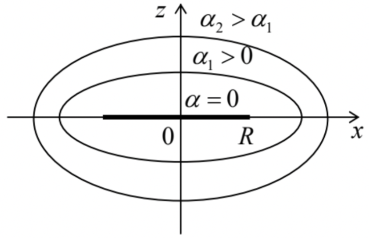
\(\newcommand{\avec}{\mathbf a}\) \(\newcommand{\bvec}{\mathbf b}\) \(\newcommand{\cvec}{\mathbf c}\) \(\newcommand{\dvec}{\mathbf d}\) \(\newcommand{\dtil}{\widetilde{\mathbf d}}\) \(\newcommand{\evec}{\mathbf e}\) \(\newcommand{\fvec}{\mathbf f}\) \(\newcommand{\nvec}{\mathbf n}\) \(\newcommand{\pvec}{\mathbf p}\) \(\newcommand{\qvec}{\mathbf q}\) \(\newcommand{\svec}{\mathbf s}\) \(\newcommand{\tvec}{\mathbf t}\) \(\newcommand{\uvec}{\mathbf u}\) \(\newcommand{\vvec}{\mathbf v}\) \(\newcommand{\wvec}{\mathbf w}\) \(\newcommand{\xvec}{\mathbf x}\) \(\newcommand{\yvec}{\mathbf y}\) \(\newcommand{\zvec}{\mathbf z}\) \(\newcommand{\rvec}{\mathbf r}\) \(\newcommand{\mvec}{\mathbf m}\) \(\newcommand{\zerovec}{\mathbf 0}\) \(\newcommand{\onevec}{\mathbf 1}\) \(\newcommand{\real}{\mathbb R}\) \(\newcommand{\twovec}[2]{\left[\begin{array}{r}#1 \\ #2 \end{array}\right]}\) \(\newcommand{\ctwovec}[2]{\left[\begin{array}{c}#1 \\ #2 \end{array}\right]}\) \(\newcommand{\threevec}[3]{\left[\begin{array}{r}#1 \\ #2 \\ #3 \end{array}\right]}\) \(\newcommand{\cthreevec}[3]{\left[\begin{array}{c}#1 \\ #2 \\ #3 \end{array}\right]}\) \(\newcommand{\fourvec}[4]{\left[\begin{array}{r}#1 \\ #2 \\ #3 \\ #4 \end{array}\right]}\) \(\newcommand{\cfourvec}[4]{\left[\begin{array}{c}#1 \\ #2 \\ #3 \\ #4 \end{array}\right]}\) \(\newcommand{\fivevec}[5]{\left[\begin{array}{r}#1 \\ #2 \\ #3 \\ #4 \\ #5 \\ \end{array}\right]}\) \(\newcommand{\cfivevec}[5]{\left[\begin{array}{c}#1 \\ #2 \\ #3 \\ #4 \\ #5 \\ \end{array}\right]}\) \(\newcommand{\mattwo}[4]{\left[\begin{array}{rr}#1 \amp #2 \\ #3 \amp #4 \\ \end{array}\right]}\) \(\newcommand{\laspan}[1]{\text{Span}\{#1\}}\) \(\newcommand{\bcal}{\cal B}\) \(\newcommand{\ccal}{\cal C}\) \(\newcommand{\scal}{\cal S}\) \(\newcommand{\wcal}{\cal W}\) \(\newcommand{\ecal}{\cal E}\) \(\newcommand{\coords}[2]{\left\{#1\right\}_{#2}}\) \(\newcommand{\gray}[1]{\color{gray}{#1}}\) \(\newcommand{\lgray}[1]{\color{lightgray}{#1}}\) \(\newcommand{\rank}{\operatorname{rank}}\) \(\newcommand{\row}{\text{Row}}\) \(\newcommand{\col}{\text{Col}}\) \(\renewcommand{\row}{\text{Row}}\) \(\newcommand{\nul}{\text{Nul}}\) \(\newcommand{\var}{\text{Var}}\) \(\newcommand{\corr}{\text{corr}}\) \(\newcommand{\len}[1]{\left|#1\right|}\) \(\newcommand{\bbar}{\overline{\bvec}}\) \(\newcommand{\bhat}{\widehat{\bvec}}\) \(\newcommand{\bperp}{\bvec^\perp}\) \(\newcommand{\xhat}{\widehat{\xvec}}\) \(\newcommand{\vhat}{\widehat{\vvec}}\) \(\newcommand{\uhat}{\widehat{\uvec}}\) \(\newcommand{\what}{\widehat{\wvec}}\) \(\newcommand{\Sighat}{\widehat{\Sigma}}\) \(\newcommand{\lt}{<}\) \(\newcommand{\gt}{>}\) \(\newcommand{\amp}{&}\) \(\definecolor{fillinmathshade}{gray}{0.9}\)Since the cylindrical and spherical coordinates used above are only the simplest examples of the curvilinear orthogonal (or just “orthogonal”) coordinates, this methodology may be extended to other coordinate systems of this type. As an example, let us calculate the self-capacitance of a thin, round conducting disk. The cylindrical or spherical coordinates would not give too much help here, because while they have the appropriate axial symmetry, they would make the boundary condition on the disk too complicated: involving two coordinates, either \(\ \rho\) and \(\ z\), or \(\ r\) and \(\ \theta\). The help comes from noting that the flat disk, i.e. the area \(\ z=0\), \(\ r<R\), may be viewed as the limiting case of an axially-symmetric ellipsoid (or “degenerate ellipsoid”, or “ellipsoid of rotation”, or “spheroid”) – the result of the rotation of the usual ellipse about one of its axes – in our case, the symmetry axis of the conducting disk – in Fig. 8, the z-axis.
Analytically, this ellipsoid may be described by the following equation:
\[\ \frac{x^{2}+y^{2}}{a^{2}}+\frac{z^{2}}{b^{2}}=1,\tag{2.58}\]
where \(\ a\) and \(\ b\) are the so-called major semi-axes, whose ratio determines ellipse’s eccentricity – the degree of its “squeezing”. For our problem, we will only need oblate ellipsoids with \(\ a \geq b\); according to Eq. (58), they may be represented as surfaces of constant \(\ \alpha\) in the degenerate ellipsoidal (or “spheroidal”) coordinates \(\ \{\alpha, \beta, \varphi\}\), which are related to the Cartesian coordinates as follows:
\[\ \begin{aligned}
&x=R \cosh \alpha \sin \beta \cos \varphi, \\
&y=R \cosh \alpha \sin \beta \sin \varphi, \\
&z=R \sinh \alpha \cos \beta .
\end{aligned}\tag{2.59}\]
Such ellipsoidal coordinates are an evident generalization of the spherical coordinates that correspond to the limit \(\ \alpha \gg1\) (i.e. \(\ r \gg R\)). In the opposite limit, the surface of constant \(\ \alpha=0\) describes our thin disk of radius \(\ R\), with the coordinate \(\ \beta\) describing the distance \(\ \rho \equiv\left(x^{2}+y^{2}\right)^{1 / 2}=R \sin \beta\) of its point from the z-axis. It is almost evident (and easy to prove) that the curvilinear coordinates (59) are also orthogonal, so that the Laplace operator may be expressed as a sum of three independent terms:
\[\ \nabla^{2}=\frac{1}{R^{2}\left(\cosh ^{2} \alpha-\sin ^{2} \beta\right)} \times\left[\begin{array}{l}
\frac{1}{\cosh \alpha} \frac{\partial}{\partial \alpha}\left(\cosh \alpha \frac{\partial}{\partial \alpha}\right) \\
+\frac{1}{\sin \beta} \frac{\partial}{\partial \beta}\left(\sin \beta \frac{\partial}{\partial \beta}\right)+\left(\frac{1}{\sin ^{2} \beta}-\frac{1}{\cosh ^{2} \alpha}\right) \frac{\partial^{2}}{\partial \varphi^{2}}
\end{array}\right].\tag{2.60}\]
Though this expression may look a bit intimidating, let us notice that in our current problem, the boundary conditions depend only on \(\ \alpha\):22
\[\ \left.\phi\right|_{\alpha=0}=V,\left.\quad \phi\right|_{\alpha=\infty}=0.\tag{2.61}\]
Hence there is every reason to assume that the electrostatic potential in all space is a function of \(\ \alpha\) alone; in other words, that all ellipsoids \(\ \alpha=\mathrm{const}\) are the equipotential surfaces. Indeed, acting on such a function \(\ \phi(\alpha)\) by the Laplace operator (60), we see that the two last terms in the square brackets vanish, and the Laplace equation (35) is reduced to a simple ordinary differential equation
\[\ \frac{d}{d \alpha}\left[\cosh \alpha \frac{d \phi}{d \alpha}\right]=0.\tag{2.62}\]
Integrating it twice, just as we did in the three previous problems, we get
\[\ \phi(\alpha)=c_{1} \int \frac{d \alpha}{\cosh \alpha}.\tag{2.63}\]
This integral may be readily worked out using the substitution \(\ \xi \equiv \sinh \alpha\) (which gives \(\ d \xi \equiv \cosh \alpha d \alpha\), \(\ \cosh ^{2} \alpha=1+\sinh ^{2} \alpha \equiv 1+\xi^{2}\)):
\[\ \phi(\alpha)=c_{1} \int_{0}^{\sinh \alpha} \frac{d \xi}{1+\xi^{2}}+c_{2}=c_{1} \tan ^{-1}(\sinh \alpha)+c_{2}.\tag{2.64}\]
The integration constants \(\ c_{1,2}\) may be simply found from the boundary conditions (61), and we arrive at the following final expression for the electrostatic potential:
\[\ \phi(\alpha)=V\left[1-\frac{2}{\pi} \tan ^{-1}(\sinh \alpha)\right].\tag{2.65}\]
This solution satisfies both the Laplace equation and the boundary conditions. Mathematicians tell us that the solution of any boundary problem of the type (35) is unique, so we do not need to look any further.
Now we may use Eq. (3) to find the surface density of electric charge, but in the case of a thin disk, it is more natural to add up such densities on its top and bottom surfaces at the same distance \(\ \rho=\left(x^{2}+y^{2}\right)^{1 / 2}\) from the disk’s center (which are evidently equal, due to the problem symmetry about the plane \(\ z=0\)): \(\ \sigma=\left.2 \varepsilon_{0} E_{n}\right|_{z=+0}\). According to Eq. (65), and the last of Eqs. (59), the electric field on the upper surface is
\[\ E_{n \mid \alpha=+0}=-\left.\frac{\partial \phi}{\partial z}\right|_{z=+0}=-\left.\frac{\partial \phi(\alpha)}{\partial(R \sinh \alpha \cos \beta)}\right|_{\alpha=+0}=\frac{2}{\pi} V \frac{1}{R \cos \beta}=\frac{2}{\pi} V \frac{1}{\left(R^{2}-\rho^{2}\right)^{1 / 2}},\tag{2.66}\]
and we see that the charge is distributed over the disk very nonuniformly:
\[\ \sigma=\frac{4}{\pi} \varepsilon_{0} V \frac{1}{\left(R^{2}-\rho^{2}\right)^{1 / 2}},\tag{2.67}\]
with a singularity at the disk edge. Below we will see that such singularities are very typical for sharp edges of conductors.23 Fortunately, in our current case the divergence is integrable, giving a finite disk charge:
\[\ Q=\int_{\text {disk } \atop \text { surface }} \sigma d^{2} \rho=\int_{0}^{R} \sigma(\rho) 2 \pi \rho d \rho=\frac{4}{\pi} \varepsilon_{0} V \int_{0}^{R} \frac{2 \pi \rho d \rho}{\left(R^{2}-\rho^{2}\right)^{1 / 2}}=4 \varepsilon_{0} V R \int_{0}^{1} \frac{d \xi}{(1-\xi)^{1 / 2}}=8 \varepsilon_{0} R V.\tag{2.68}\]
Thus, for the disk’s self-capacitance we get a very simple result,
C: Round disk
\[\ C=8 \varepsilon_{0} R \equiv \frac{2}{\pi} 4 \pi \varepsilon_{0} R,\tag{2.69}\]
a factor of \(\ \pi / 2 \approx 1.57\) lower than that for the conducting sphere of the same radius, but still complying with the general estimate (18).
Can we always find such a “good” system of orthogonal coordinates? Unfortunately, the answer is no, even for highly symmetric geometries. This is why the practical value of this approach is limited, and other, more general methods of boundary problem solution are clearly needed. Before proceeding to their discussion, however, let me note that in the case of 2D problems (i.e. cylindrical geometries24), the orthogonal coordinate method gets much help from the following conformal mapping approach.
Let us consider a pair of Cartesian coordinates \(\ \{x, y\}\) of the cross-section plane as a complex variable \(\ z \equiv x+i y\),25 where \(\ i\) is the imaginary unit \(\ \left(i^{2}=-1\right)\), and let \(\ u d(z)=u+i v\) be an analytic complex function of \(\ z\).26 For our current purposes, the most important property of an analytic function is that its real and imaginary parts obey the following Cauchy-Riemann relations:27
\[\ \frac{\partial u}{\partial x}=\frac{\partial v}{\partial y}, \quad \frac{\partial v}{\partial x}=-\frac{\partial u}{\partial y}.\tag{2.70}\]
For example, for the function
\[\ \boldsymbol{\omega}=\boldsymbol{z}^{2} \equiv(x+i y)^{2}=\left(x^{2}-y^{2}\right)+2 i x y,\tag{2.71}\]
whose real and imaginary parts are
\[\ u \equiv \operatorname{Re} \boldsymbol{\omega}=x^{2}-y^{2}, \quad v \equiv \operatorname{Im} \boldsymbol{\omega}=2 x y,\tag{2.72}\]
we immediately see that \(\ \partial u / \partial x=2 x=\partial v / \partial y\), and \(\ \partial v / \partial x=2 y=-\partial u / \partial y\), in accordance with Eq. (70).
Let us differentiate the first of Eqs. (70) over x again, then change the order of differentiation, and after that use the latter of those equations:
\[\ \frac{\partial^{2} u}{\partial x^{2}}=\frac{\partial}{\partial x} \frac{\partial u}{\partial x}=\frac{\partial}{\partial x} \frac{\partial v}{\partial y}=\frac{\partial}{\partial y} \frac{\partial v}{\partial x}=-\frac{\partial}{\partial y} \frac{\partial u}{\partial y}=-\frac{\partial^{2} u}{\partial y^{2}},\tag{2.73}\]
and similarly for \(\ v\). This means that the sum of second-order partial derivatives of each of the real functions \(\ u(x, y)\) and \(\ v(x, y)\) is zero, i.e. that both functions obey the 2D Laplace equation. This mathematical fact opens a nice way of solving problems of electrostatics for (relatively simple) 2D geometries. Imagine that for a particular boundary problem we have found a function \(\ \boldsymbol{\omega(z)}\) for that either \(\ u(x, y)\) or \(\ v(x, y)\) is constant on all electrode surfaces. Then all lines of constant \(\ u\) (or \(\ v\)) represent equipotential surfaces, i.e. the problem of the potential distribution has been essentially solved.
As a simple example, let us consider a problem important for practice: the quadrupole electrostatic lens – a system of four cylindrical electrodes with hyperbolic cross-sections, whose boundaries obey the following relations:
\[\ x^{2}-y^{2}= \begin{cases}+a^{2}, & \text { for the left and right electrodes, } \\ -a^{2}, & \text { for the top and bottom electrodes, }\end{cases}\tag{2.74}\]
voltage-biased as shown in Fig. 9a.
 Fig. 2.9. (a) The quadrupole electrostatic lens’ cross-section and (b) its conformal mapping.
Comparing these relations with Eqs. (72), we see that each electrode surface corresponds to a constant value of the real part \(\ u(x, y)\) of the function (71): \(\ u=\pm a^{2}\). Moreover, the potentials of both surfaces with \(\ u=+a^{2}\) are equal to \(\ +V / 2\), while those with \(\ u=-a^{2}\) are equal to \(\ -V / 2\). Hence we may conjecture that the electrostatic potential at each point is a function of u alone; moreover, a simple linear function,
\[\ \phi=c_{1} u+c_{2}=c_{1}\left(x^{2}-y^{2}\right)+c_{2},\tag{2.75}\]
is a valid (and hence the unique) solution of our boundary problem. Indeed, it does satisfy the Laplace equation, while the constants \(\ c_{1,2}\) may be readily selected in a way to satisfy all the boundary conditions shown in Fig. 9a:
\[\ \phi=\frac{V}{2} \frac{x^{2}-y^{2}}{a^{2}}\tag{2.76}\]
so that the boundary problem has been solved.
According to Eq. (76), all equipotential surfaces are hyperbolic cylinders, similar to those of the electrode surfaces. What remains is to find the electric field at an arbitrary point inside the system:
\[\ E_{x}=-\frac{\partial \phi}{\partial x}=-V \frac{x}{a^{2}}, \quad E_{y}=-\frac{\partial \phi}{\partial y}=V \frac{y}{a^{2}}.\tag{2.77}\]
These formulas show, in particular, that if charged particles (e.g., electrons in an electron-optics system) are launched to fly ballistically through such a lens, along the z-axis, they experience a force pushing them toward the symmetry axis and proportional to the particle’s deviation from the axis (and thus equivalent in action to an optical lens with a positive refraction power) in one direction, and a force pushing them out (negative refractive power) in the perpendicular direction. One can show that letting the particles fly through several such lenses, with alternating voltage polarities, in series, enables beam focusing.28
Hence, we have reduced the 2D Laplace boundary problem to that of finding the proper analytic function \(\ \boldsymbol{w(z)}\). This task may be also understood as that of finding a conformal map, i.e. a correspondence between components of any point pair, \(\ \{x, y\}\) and \(\ \{u, v\}\), residing, respectively, on the initial Cartesian plane \(\ \boldsymbol{z}\) and the plane \(\ \boldsymbol{w}\) of the new variables. For example, Eq. (71) maps the real electrode configuration onto a plane capacitor of an infinite area (Fig. 9b), and the simplicity of Eq. (75) is due to the fact that for the latter system the equipotential surfaces are just parallel planes \(\ u=\mathrm{const}\).
For more complex geometries, the suitable analytic function \(\ \boldsymbol{\omega(z)}\) may be hard to find. However, for conductors with piece-linear cross-section boundaries, substantial help may be obtained from the following Schwarz-Christoffel integral
\[\ \boldsymbol{w(z)}=\text { const } \times \int \frac{d \boldsymbol{z}}{\left(\boldsymbol{z}-x_{1}\right)^{k_{1}}\left(\boldsymbol{z}-x_{2}\right)^{k_{2}} \ldots\left(\boldsymbol{z}-x_{N-1}\right)^{k_{N-1}}}.\tag{2.78}\]
that provides a conformal mapping of the interior of an arbitrary N-sided polygon on the plane \(\ \boldsymbol{\omega}=u+iv\), onto the upper-half (y > 0) of the plane \(\ \boldsymbol{z}=x+i y\). In Eq. (78), \(\ x_{j}(j=1,2, N-1)\) are the points of the y = 0 axis (i.e., of the boundary of the mapped region on plane \(\ \boldsymbol{z}\)) to which the corresponding polygon vertices are mapped, while \(\ k_{j}\) are the exterior angles at the polygon vertices, measured in the units of \(\ \pi\), with \(\ -1 \leq k_{j} \leq+1\) – see Fig. 10.29 Of the points \(\ x_{j}\), two may be selected arbitrarily (because their effects may be compensated by the multiplicative constant in Eq. (78), and the additive constant of integration), while all the others have to be adjusted to provide the correct mapping.
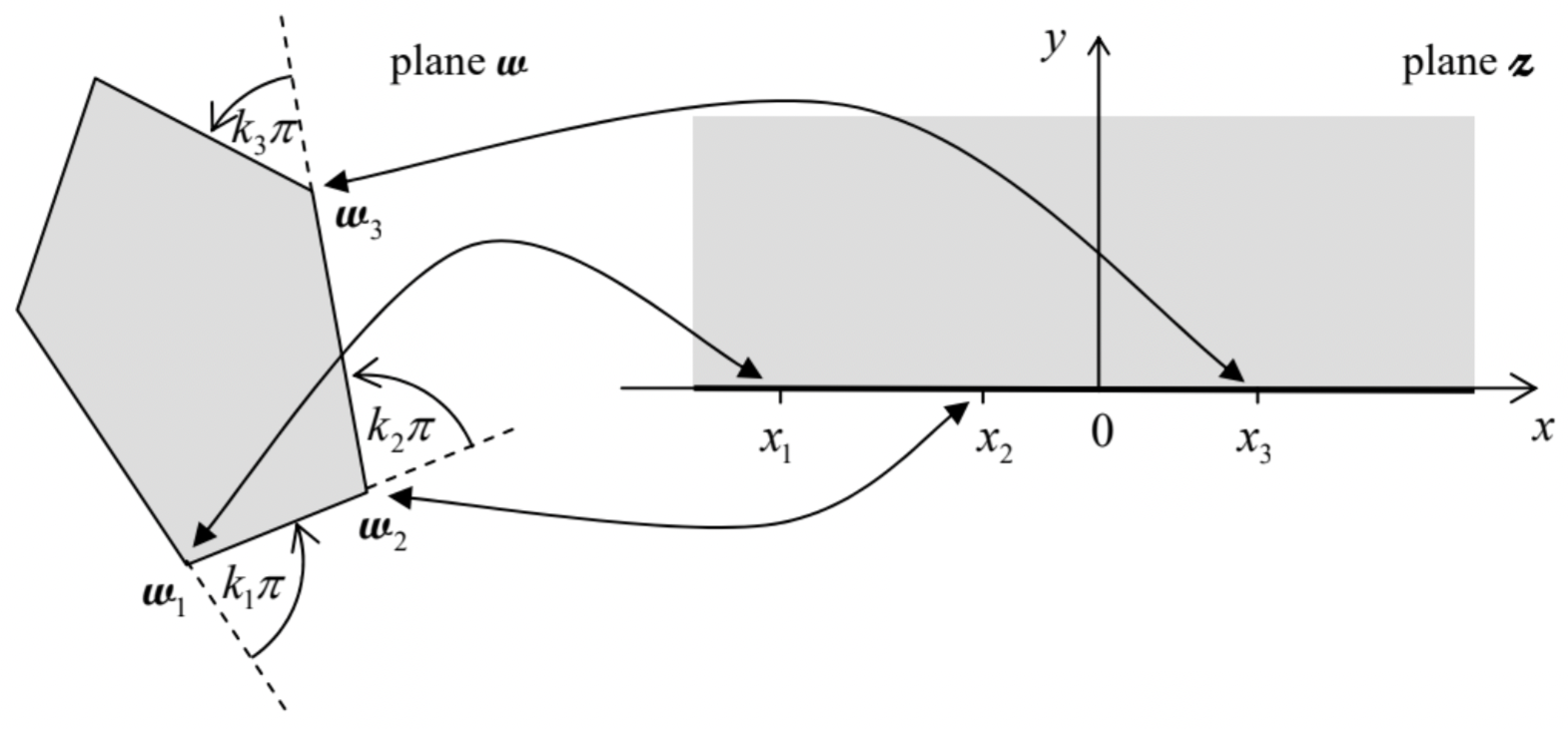 Fig. 2.10. The Schwartz-Christoffel mapping of a polygon’s interior onto the upper half-plane.
In the general case, the complex integral (78) may be hard to tackle. However, in some important cases, in particular those with right angles \(\ \left(k_{j}=\pm 1 / 2\right)\) and/or with some points \(\ \boldsymbol{w}_{j}\) at infinity, the integrals may be readily worked out, giving explicit analytical expressions for the mapping functions \(\ \boldsymbol{\omega(z)}\). For example, let us consider a semi-infinite strip, defined by restrictions \(\ -1 \leq u \leq+1\) and \(\ 0 \leq v\), on the plane \(\ \boldsymbol{w}\) – see the left panel of Fig. 11.
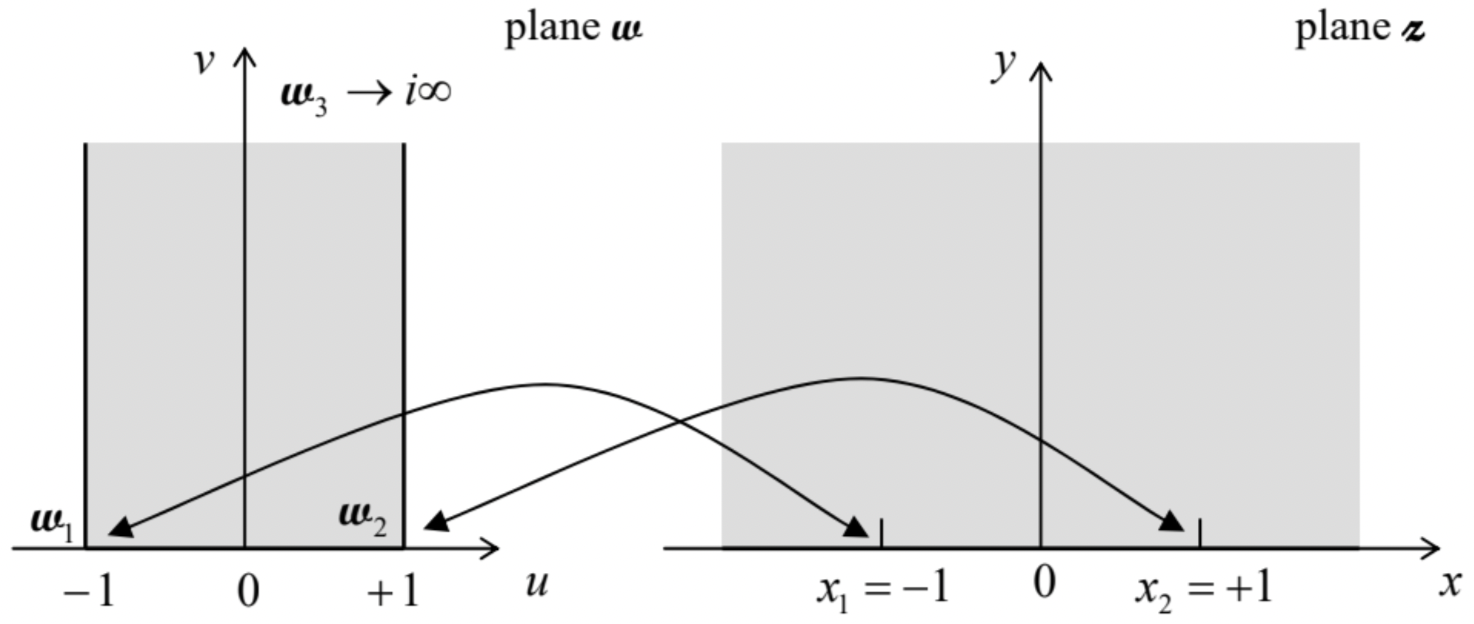
The strip may be considered as a triangle, with one vertex at the infinitely distant vertical point \(\ \boldsymbol{\omega}_{3}=0+i \infty\). Let us map the polygon on the upper half of plane \(\ \boldsymbol{z}\), shown on the right panel of Fig. 11, with the vertex \(\ \boldsymbol{w}_{1}=-1+i 0\) mapped onto the point \(\ \boldsymbol{z}_{1}=-1+i 0\), and the vertex \(\ \boldsymbol{w}_{2}=+1+i 0\) mapped onto the point \(\ \boldsymbol{z}_{2}=+1+i 0\). Since the external angles at both these vertices are equal to \(\ +\pi / 2\), and hence \(\ k_{1}=k_{2}=+{1\over2}\), Eq. (78) is reduced to
\[\ \boldsymbol{w(z)}=\text { const } \times \int \frac{d z}{(z+1)^{1 / 2}(z-1)^{1 / 2}} \equiv \text { const } \times \int \frac{d z}{\left(z^{2}-1\right)^{1 / 2}} \equiv \text { const } \times i \int \frac{d z}{\left(1-z^{2}\right)^{1 / 2}}.\tag{2.79}\]
This complex integral may be worked out, just as for real \(\ \boldsymbol{z}\), with the substitution \(\ \boldsymbol{z}=\sin \xi\), giving
\[\ \boldsymbol{w(z)}=\text { const' } \times \int^{\sin ^{-1} \boldsymbol{z}} d \xi=c_{1} \sin ^{-1} \boldsymbol{z}+c_{2}.\tag{2.80}\]
Determining the constants \(\ c_{1,2}\) from the required mapping, i.e. from the conditions \(\ \boldsymbol{w}(-1+i 0)=-1+i 0\) and \(\ \boldsymbol{w}(+1+i 0)=+1+i 0\) (see the arrows in Fig. 11), we finally get
\[\ \boldsymbol{w(z})=\frac{2}{\pi} \sin ^{-1} \boldsymbol{z}, \quad \text { i.e. } \boldsymbol{z}=\sin \frac{\pi \boldsymbol{w}}{2}.\tag{2.81a}\]
Using the well-known expression for the sine of a complex argument,30 we may rewrite this elegant result in either of the following two forms for the real and imaginary components of \(\ \boldsymbol{z}\) and \(\ \boldsymbol{w}\):
\[\ \begin{gathered}
u=\frac{2}{\pi} \sin ^{-1} \frac{2 x}{\left[(x+1)^{2}+y^{2}\right]^{1 / 2}+\left[(x-1)^{2}+y^{2}\right]^{1 / 2}}, \quad v=\frac{2}{\pi} \cosh ^{-1} \frac{\left[(x+1)^{2}+y^{2}\right]^{1 / 2}+\left[(x-1)^{2}+y^{2}\right]^{1 / 2}}{2}, \\
x=\sin \frac{\pi u}{2} \cosh \frac{\pi v}{2}, \quad y=\cos \frac{\pi u}{2} \sinh \frac{\pi v}{2}.
\end{gathered}\tag{2.81b}\]
It is amazing how perfectly does the last formula manage to keep \(\ y \equiv 0\) at the different borders of our \(\ \boldsymbol{w}\)-region (Fig. 11): at its side borders \(\ (u=\pm 1,0 \leq v<\infty)\), this is performed by the first multiplier, while at the bottom border \(\ (-1 \leq u \leq+1, v=0)\), the equality is enforced by the second multiplier.
This mapping may be used to solve several electrostatics problems with the geometry shown in Fig. 11a; probably the most surprising of them is the following one. A straight gap of width \(\ 2t\) is cut in a very thin conducting plane, and voltage V is applied between the resulting half-planes – see the bold straight lines in Fig. 12.
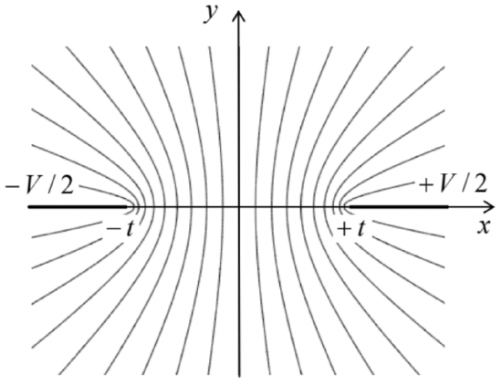 Fig. 2.12. The equipotential surfaces of the electric field between two thin conducting semi-planes (or rather their cross-sections by the plane z = const).
Selecting a Cartesian coordinate system with the z-axis directed along the cut, the y-axis normal to the plane, and the origin in the middle of the cut (Fig. 12), we can write the boundary conditions of this Laplace problem as
\[\ \phi= \begin{cases}+V / 2, & \text { for } x>+t, y=0, \\ -V / 2, & \text { for } x<-t, y=0.\end{cases}\tag{2.82}\]
(Due to the problem’s symmetry, we may expect that in the middle of the gap, i.e. at \(\ -t<x<+t\) and \(\ y=0\), the electric field is parallel to the plane and hence \(\ \partial \phi / \partial y=0\).) The comparison of Figs. 11 and 12 shows that if we normalize our coordinates \(\ \{x, y\}\) to \(\ t\), Eqs. (81) provide the conformal mapping of our system on the plane \(\ \boldsymbol{z}\) to the plane capacitor on the plane \(\ \boldsymbol{w}\), with the voltage \(\ V\) between two planes \(\ u=\pm 1\). Since we already know that in that case \(\ \phi=(V / 2) u\), we may immediately use the first of Eqs. (81b) to write the final solution of the problem:31
\[\ \phi=\frac{V}{2} u=\frac{V}{\pi} \sin ^{-1} \frac{2 x}{\left[(x+t)^{2}+y^{2}\right]^{1 / 2}+\left[(x-t)^{2}+y^{2}\right]^{1 / 2}}.\tag{2.83}\]
The thin lines in Fig. 12 show the corresponding equipotential surfaces;32 it is evident that the electric field concentrates at the gap edges, just as it did at the edge of the thin disk (Fig. 8). Let me leave the remaining calculation of the surface charge distribution and the mutual capacitance between the half-planes (per unit length) for the reader’s exercise.
Reference
22 I have called the disk’s potential \(\ V\), to distinguish it from the potential \(\ \phi\) at an arbitrary point of space.
23 If you seriously worry about the formal infinity of the charge density at \(\ \rho \rightarrow R\), please remember that this mathematical artifact disappears with the account of nonzero thickness of the disk.
24 Let me remind the reader that the term cylindrical describes any surface formed by a translation, along a straight line, of an arbitrary curve, and hence more general than the usual circular cylinder. (In this terminology, for example, a prism is also a cylinder of a particular type, formed by a translation of a polygon.)
25 The complex variable \(\ \boldsymbol{z}\) should not be confused with the (real) 3rd spatial coordinate z! We are considering 2D problems now, with the potential independent of z.
26 An analytic (or "holomorphic") function may be defined as the one that may be expanded into the Taylor series in its complex argument, i.e. is infinitely differentiable in the given point. (Almost all “regular” functions, such as \(\ \boldsymbol{z}^{n}, \boldsymbol{z}^{1 / n}, \exp \boldsymbol{z}, \ln \boldsymbol{z}\), etc., and their combinations are analytic at all \(\ \boldsymbol{z}\), maybe besides certain special points.) If the reader needs to brush up their background on this subject, I can recommend a popular textbook by M. Spiegel et al., Complex Variables, 2nd ed., McGraw-Hill, 2009.
27 These relations may be used, in particular, to prove the Cauchy integral formula – see, e.g., MA Eq. (15.1).
28 See, e.g., textbook by P. Grivet, Electron Optics, 2nd ed., Pergamon, 1972, or the review collection A. Septier (ed.), Focusing Charged Particles, vol. I, Academic Press, 1967, in particular the review by K.-J. Hanszen and R. Lauer on pp. 251-307 of this collection.
29 The integral (78) includes only \(\ (N-1)\) rather than \(\ N\) poles because a polygon’s shape is fully determined by \(\ (N–1)\) positions \(\ \boldsymbol{w}_{j}\) of its vertices and \(\ (N – 1)\) angles \(\ \pi k_{j}\). In particular, since the algebraic sum of all external angles of a polygon equals \(\ 2 \pi\), the last angle parameter \(\ k_{j}=k_{N}\) is uniquely determined by the set of the previous ones.
30 See, e.g., MA Eq. (3.5).
31 This result may be also obtained using the so-called elliptical (not ellipsoidal!) coordinates, and by the Green’s function method, to be discussed in Sec. 10 below.
32 Another graphical representation of the electric field distribution, by field lines, is less convenient. (It is more useful for the magnetic field, so there is no surprise that the field lines were introduced only by Michael Faraday in the 1830s.) As a reminder, the field lines are defined as the curves to which the field vectors are tangential at each point. Hence the electric field lines are always normal to the equipotential surfaces, so that it is always straightforward to sketch them, if desirable, from the equipotential surface pattern – like the one shown in Fig. 12.