3.1: Electric Dipole

Let us consider a localized system of charges, of a linear size scale \(\ a\), and derive a simple but approximate expression for the electrostatic field induced by the system at a distant point \(\ \mathbf{r}\). For that, let us select a reference frame with the origin either somewhere inside the system, or at a distance of the order of \(\ a\) from it (Fig. 1).

Fig. 3.1. Deriving the approximate expression for the electrostatic field of a localized system of charges at a distant point \(\ \left(r>>r^{\prime} \sim a\right)\).

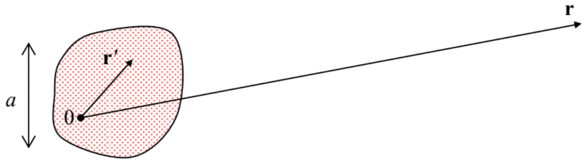
Then positions of all charges of the system satisfy the following condition:

\[\ r^{\prime}<<r.\tag{3.1}\]

Using this condition, we can expand the general expression (1.38) for the electrostatic potential \(\ \phi(\mathbf{r})\) of the system into the Taylor series in small parameter \(\ \mathbf{r}^{\prime}\). For any function of type \(\ f\left(\mathbf{r}-\mathbf{r}^{\prime}\right)\), the expansion may be represented as¹

\[\ f\left(\mathbf{r}-\mathbf{r}^{\prime}\right)=f(\mathbf{r})-\sum_{j=1}^{3} r_{j}^{\prime} \frac{\partial f}{\partial r_{j}}(\mathbf{r})+\frac{1}{2 !} \sum_{j, j^{\prime}=1}^{3} r_{j}^{\prime} r_{j^{\prime}}^{\prime} \frac{\partial^{2} f}{\partial r_{j} \partial r_{j^{\prime}}}(\mathbf{r})-\ldots.\tag{3.2}\]

Applying this formula to the free-space Green’s function \(\ 1 /\left|\mathbf{r}-\mathbf{r}^{\prime}\right|\) in Eq. (1.38), we get the so-called multipole expansion of the electrostatic potential:

\[\ \phi(\mathbf{r})=\frac{1}{4 \pi \varepsilon_{0}}\left(\frac{1}{r} Q+\frac{1}{r^{3}} \sum_{j=1}^{3} r_{j} p_{j}+\frac{1}{2 r^{5}} \sum_{j, j^{\prime}=1}^{3} r_{j} r_{j^{\prime}}\mathscr{Q}_{j j^{\prime}}+\ldots\right),\tag{3.3}\]

whose \(\ \mathbf{r}\)-independent parameters are defined as follows:

\[\ Q \equiv \int \rho\left(\mathbf{r}^{\prime}\right) d^{3} r^{\prime}, \quad p_{j} \equiv \int \rho\left(\mathbf{r}^{\prime}\right) r_{j}^{\prime} d^{3} r^{\prime}, \quad \mathscr{Q}_{j j^{\prime}} \equiv \int \rho\left(\mathbf{r}^{\prime}\right)\left(3 r_{j}^{\prime} r_{j^{\prime}}{ }^{\prime}-r^{\prime 2} \delta_{j j^{\prime}}\right) d^{3} r^{\prime}.\tag{3.4}\]

(Indeed, the two leading terms of the expansion (2) may be rewritten in the vector form \(\ f(\mathbf{r})-\mathbf{r}^{\prime} \cdot \nabla f(\mathbf{r})\), and the gradient of such a spherically-symmetric function \(\ f(r)=1 / r\) is just \(\ \mathbf{n}_{r} d f / d r\), so that

\[\ \frac{1}{\left|\mathbf{r}-\mathbf{r}^{\prime}\right|} \approx \frac{1}{r}-\mathbf{r}^{\prime} \cdot \mathbf{n}_{r} \frac{d}{d r}\left(\frac{1}{r}\right)=\frac{1}{r}+\mathbf{r}^{\prime} \cdot \frac{\mathbf{r}}{r^{3}},\tag{3.5}\]

immediately giving the two first terms of Eq. (3). The proof of the third, quadrupole term in Eq. (3) is similar but a bit longer, and is left for the reader’s exercise.)

Evidently, the scalar parameter \(\ Q\) in Eqs. (3)-(4) is just the total charge of the system. The constants \(\ p_{j}\) may be considered as Cartesian components of the following vector:

Electric dipole moment

\[\ \mathbf{p} \equiv \int \rho\left(\mathbf{r}^{\prime}\right) \mathbf{r}^{\prime} d^{3} r^{\prime},\tag{3.6}\]

called the system’s electric dipole moment, and \(\ \mathcal{Q}_{j j^{\prime}}\) are the Cartesian components of a tensor – system’s electric quadrupole moment. If \(\ Q \neq 0\), all higher terms on the right-hand side of Eq. (3), at large distances (1), are just small corrections to the first one, and in many cases may be ignored. However, the net charge of many systems is exactly zero, the most important examples being neutral atoms and molecules. For such neural systems, the second (dipole-moment) term in Eq. (3) is, most frequently, the leading one. (Such systems are called electric dipoles.) Due to its importance, let us rewrite the expression for this term in three other, mathematically equivalent forms:

Electric dipole’s potential

\[\ \phi_{\mathrm{d}} \equiv \frac{1}{4 \pi \varepsilon_{0}} \frac{\mathbf{r} \cdot \mathbf{p}}{r^{3}} \equiv \frac{1}{4 \pi \varepsilon_{0}} \frac{p \cos \theta}{r^{2}} \equiv \frac{1}{4 \pi \varepsilon_{0}} \frac{p z}{\left(x^{2}+y^{2}+z^{2}\right)^{3 / 2}},\tag{3.7}\]

that are more convenient for some applications. Here \(\ \theta\) is the angle between the vectors \(\ \mathbf{p}\) and \(\ \mathbf{r}\), and in the last (Cartesian) representation, the z-axis is directed along the vector \(\ \mathbf{p}\). Fig. 2a shows equipotential surfaces of the dipole field – or rather their cross-sections by any plane in which the vector \(\ \mathbf{p}\) resides.

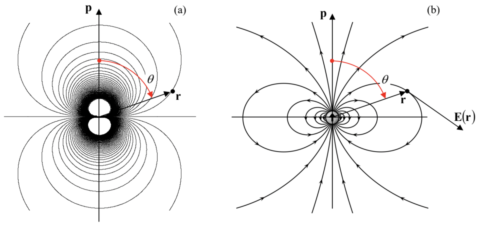Fig. 3.2. (a) The equipotential surfaces and (b) the electric field lines of a dipole. (Panel (b) adapted from http://en.Wikipedia.org/wiki/Dipole under the GNU Free Documentation License.)

The simplest example of a system whose field, at large distances, approaches the dipole field (7), is two equal but opposite point charges (“poles”), \(\ +q\) and \(\ -q\), with the radius-vectors, respectively, \(\ \mathbf{r}_{+}\) and \(\ \mathbf{r}_{-}\):

\[\ \rho(\mathbf{r})=(+q) \delta\left(\mathbf{r}-\mathbf{r}_{+}\right)+(-q) \delta\left(\mathbf{r}-\mathbf{r}_{-}\right).\tag{3.8}\]

For this system (sometimes called the physical dipole), Eq. (4) yields

\[\ \mathbf{p}=(+q) \mathbf{r}_{+}+(-q) \mathbf{r}_{-}=q\left(\mathbf{r}_{+}-\mathbf{r}_{-}\right)=q \mathbf{a},\tag{3.9}\]

where \(\ \mathbf{a}\) is the vector connecting the points \(\ \mathbf{r}_{-}\) and \(\ \mathbf{r}_{+}\). Note that in this case (and indeed for all systems with \(\ Q=0\)), the dipole moment does not depend on the choice of the reference frame’s origin.

A less trivial example of a dipole is a conducting sphere of radius \(\ R\) in a uniform external electric field \(\ \mathbf{E}_{0}\). As a reminder, this problem was solved in Sec. 2.8, and its result is expressed by Eq. (2.176). The first term in the parentheses of that relation describes just the external field (2.173), so that the field of the sphere itself (i.e. that of the surface charge induced by \(\ \mathbf{E}_{0}\)) is given by the second term:

\[\ \phi_{\mathrm{s}}=\frac{E_{0} R^{3}}{r^{2}} \cos \theta.\tag{3.10}\]

Comparing this expression with the second form of Eq. (7), we see that the sphere has an induced dipole moment

\[\ \mathbf{p}=4 \pi \varepsilon_{0} \mathbf{E}_{0} R^{3}.\tag{3.11}\]

This is an interesting example of a virtually pure dipole field: at all points outside the sphere \(\ (r>R)\), the field has neither a quadrupole moment nor any higher moments.

Other examples of dipole fields are given by two more systems discussed in Chapter 2 – see Eqs. (2.215) and (2.219). Those systems, however, do have higher-order multipole moments, so that for them, Eq. (7) gives only the long-distance approximation.

Now returning to the general properties of the dipole field (7), let us calculate its characteristics. First of all, we may use Eq. (7) to calculate the electric field of a dipole:

\[\ \mathbf{E}_{\mathrm{d}}=-\nabla \phi_{\mathrm{d}}=-\frac{1}{4 \pi \varepsilon_{0}} \nabla\left(\frac{\mathbf{r} \cdot \mathbf{p}}{r^{3}}\right)=-\frac{1}{4 \pi \varepsilon_{0}} \nabla\left(\frac{p \cos \theta}{r^{2}}\right).\tag{3.12}\]

The differentiation is easiest in the spherical coordinates, using the well-known expression for the gradient of a scalar function in these coordinates² and taking the z-axis parallel to the dipole moment \(\ \mathbf{p}\). From the last form of Eq. (12), we immediately get

Electric dipole’s field

\[\ \mathbf{E}_{\mathrm{d}}=\frac{p}{4 \pi \varepsilon_{0} r^{3}}\left(2 \mathbf{n}_{r} \cos \theta+\mathbf{n}_{\theta} \sin \theta\right) \equiv \frac{1}{4 \pi \varepsilon_{0}} \frac{3 \mathbf{r}(\mathbf{r} \cdot \mathbf{p})-\mathbf{p} r^{2}}{r^{5}}.\tag{3.13}\]

Fig. 2b above shows the electric field lines given by Eqs. (13). The most important features of this result are a faster drop of the field’s magnitude (\(\ E_{\mathrm{d}} \propto 1 / r^{3}\), rather than \(\ E \propto 1 / r^{2}\) for a point charge), and the change of the signs of all field components as functions of the polar angle \(\ \theta\).

Next, let us use Eq. (1.55) to calculate the potential energy of interaction between a dipole and an external electric field. Assuming that the external field does not change much at distances of the order of \(\ a\) (Fig. 1), we may expand its potential \(\ \phi_{\mathrm{ext}}(\mathbf{r})\) into the Taylor series, and keep only its two
leading terms:

\[\ U=\int \rho(\mathbf{r}) \phi_{\text {ext }}(\mathbf{r}) d^{3} r \approx \int \rho(\mathbf{r})\left[\phi_{\text {ext }}(0)+\mathbf{r} \cdot \nabla \phi_{\text {ext }}(0)\right] d^{3} r \equiv Q \phi_{\text {ext }}(0)-\mathbf{p} \cdot \mathbf{E}_{\text {ext }}.\tag{3.14}\]

The first term is the potential energy the system would have if it were just a point charge. If the net charge \(\ Q\) is zero, that term disappears, and the leading contribution is due to the dipole moment:

\[\ U=-\mathbf{p} \cdot \mathbf{E}_{\text {ext }}, \quad \text { for } \mathbf{p}=\text { const }.\tag{3.15a}\]

Dipole’s energy in external field

Note that this result is only valid for a fixed dipole, with \(\ \mathbf{p}\) independent of \(\ \mathbf{E}_{\text {ext }}\). In the opposite limit, when the dipole is induced by the field, i.e. \(\ \mathbf{p} \propto \mathbf{E}_{\text {ext }}\) (you may have one more look at Eq. (11) to see an example of such a proportionality), we need to start with Eq. (1.60) rather than Eq. (1.55), getting

\[\ U=-\frac{1}{2} \mathbf{p} \cdot \mathbf{E}_{\text {ext }}, \quad \text { for } \mathbf{p} \propto \mathbf{E}_{\text {ext }}.\tag{3.15b}\]

In particular, combining Eqs. (13) and Eq. (15a), we may get the following important formula for the interaction of two independent dipoles:

\[\ U_{\mathrm{int}}=\frac{1}{4 \pi \varepsilon_{0}} \frac{\mathbf{p}_{1} \cdot \mathbf{p}_{2} r^{2}-3\left(\mathbf{r} \cdot \mathbf{p}_{1}\right)\left(\mathbf{r} \cdot \mathbf{p}_{2}\right)}{r^{5}}=\frac{1}{4 \pi \varepsilon_{0}} \frac{p_{1 x} p_{2 x}+p_{1 y} p_{2 y}-2 p_{1 z} p_{2 z}}{r^{3}},\tag{3.16}\]

where \(\ \mathbf{r}\) is the vector connecting the dipoles, and the z-axis is directed along this vector. It is easy to prove (this exercise is left for the reader) that if the magnitude of each dipole moment is fixed (the approximation valid, in particular, for weak interaction of so-called polar molecules), this potential energy reaches its minimum at, and hence favors the parallel orientation of the dipoles along the line connecting them. Note also that in this case, \(\ U_{\mathrm{int}}\) is proportional to \(\ 1 / r^{3}\). On the other hand, if each moment \(\ \mathbf{p}\) has a random value plus a component due to its polarization by the electric field of its counterpart: \(\ \Delta \mathbf{p}_{1,2} \propto \mathbf{E}_{2,1} \propto 1 / r^{3}\), their average interaction energy (which may be calculated from Eq. (16) with the additional factor 1⁄2) is always negative and is proportional to \(\ 1 / r^{6}\). Such negative potential describes, in particular, the long-range, attractive part (the so-called London dispersion force) of the interaction between electrically neutral atoms and molecules.³

According to Eqs. (15), to reach the minimum of \(\ U\), the electric field “tries” to align the dipole’s direction along its own. The quantitative expression of this effect is the \(\ \boldsymbol{\tau}\) exerted by the field. The simplest way to calculate it is to sum up all the elementary torques \(\ d \boldsymbol{\tau}=\mathbf{r} \times d \mathbf{F}_{\mathrm{ext}}=\mathbf{r} \times \mathbf{E}_{\mathrm{ext}}(\mathbf{r}) \rho(\mathbf{r}) d^{3} r\) exerted on all elementary charges of the system:

\[\ \boldsymbol{\tau}=\int \mathbf{r} \times \mathbf{E}_{\text {ext }}(\mathbf{r}) \rho(\mathbf{r}) d^{3} r \approx \mathbf{p} \times \mathbf{E}_{\text {ext }}(0),\tag{3.17}\]

where at the last step, the spatial dependence of the external field was again neglected. The spatial dependence of \(\ \mathbf{E}_{\mathrm{ext}}\) cannot, however, be ignored at the calculation of the total force exerted by the field on the dipole (with \(\ Q=0\)). Indeed, Eqs. (15) shows that if the field is constant, the dipole energy is the same at all spatial points, and hence the net force is zero. However, if the field has a non-zero gradient, a total force does appear; for a field-independent dipole,

\[\ \mathbf{F}=-\nabla U=\nabla\left(\mathbf{p} \cdot \mathbf{E}_{\mathrm{ext}}\right),\tag{3.18}\]

where the derivative has to be taken at the dipole’s position (in our notation, at \(\ \mathbf{r}=0\). If the dipole that is being moved in a field retains its magnitude and orientation, then the last formula is equivalent to⁴

\[\ \mathbf{F}=(\mathbf{p} \cdot \nabla) \mathbf{E}_{\text {ext }}.\tag{3.19}\]

Alternatively, the last expression may be obtained similarly to Eq. (14):

\[\ \mathbf{F}=\int \rho(\mathbf{r}) \mathbf{E}_{\mathrm{ext}}(\mathbf{r}) d^{3} r \approx \int \rho(\mathbf{r})\left[\mathbf{E}_{\mathrm{ext}}(0)+(\mathbf{r} \cdot \nabla) \mathbf{E}_{\mathrm{ext}}\right] d^{3} r=Q \mathbf{E}_{\mathrm{ext}}(0)+(\mathbf{p} \cdot \nabla) \mathbf{E}_{\mathrm{ext}}.\tag{3.20}\]

Finally, let me add a note on the so-called coarse-grain model of the dipole. The dipole approximation explored above is asymptotically correct only at large distances, \(\ r \gg a\). However, for some applications (including the forthcoming discussion of the molecular field effects in Sec. 3) it is important to have an expression that would be approximately valid everywhere in space, though maybe without exact details at \(\ r \sim a\), and also give the correct result for the space average of the electric field,

\[\ \overline{\mathbf{E}} \equiv \frac{1}{V} \int_{V} \mathbf{E} d^{3} r,\tag{3.21}\]

where \(\ V\) is a regularly-shaped volume much larger than \(\ a^{3}\), for example a sphere of a radius \(\ R \gg a\), with the dipole at its center. For the field \(\ \mathbf{E}_{\mathrm{d}}\) given by Eq. (13), such an average is zero. Indeed, let us consider the Cartesian components of that vector in a reference frame with the z-axis directed along the vector \(\ \mathbf{p}\). Due to the axial symmetry of the field, the averages of the components \(\ E_{x}\) and \(\ E_{y}\) vanish. Let us use Eq. (13) to spell out the “vertical” component of the field (parallel to the dipole moment vector):

\[\ E_{z} \equiv \mathbf{E}_{\mathrm{d}} \cdot \frac{\mathbf{p}}{p}=\frac{1}{4 \pi \varepsilon_{0} r^{3}}\left(2 \mathbf{n}_{r} \cdot \mathbf{p} \cos \theta-\mathbf{n}_{\theta} \cdot \mathbf{p} \sin \theta\right)=\frac{p}{4 \pi \varepsilon_{0} r^{3}}\left(2 \cos ^{2} \theta-\sin ^{2} \theta\right).\tag{3.22}\]

Integrating this expression over the whole solid angle \(\ \Omega=4 \pi\), at fixed \(\ r\), using a convenient variable substitution \(\ \cos \theta \equiv \xi\), we get

\[\ \oint_{4 \pi} E_{z} d \Omega=2 \pi \int_{0}^{\pi} E_{z} \sin \theta d \theta=\frac{p}{2 \varepsilon_{0} r^{3}} \int_{0}^{\pi}\left(2 \cos ^{2} \theta-\sin ^{2} \theta\right) \sin \theta d \theta=\frac{p}{2 \varepsilon_{0} r^{3}} \int_{-1}^{+1}\left(3 \xi^{2}-1\right) d \xi=0.\tag{3.23}\]

On the other hand, the exact electric field of an arbitrary charge distribution, with the total dipole moment \(\ \mathbf{p}\), obeys the following equality:

\[\ \int_{V} \mathbf{E}(\mathbf{r}) d^{3} r=-\frac{\mathbf{p}}{3 \varepsilon_{0}} \equiv-\frac{1}{4 \pi \varepsilon_{0}} \frac{4 \pi}{3} \mathbf{p},\tag{3.24}\]

where the integration is over any sphere containing all the charges. A proof of this formula for the general case requires a straightforward, but somewhat tedious integration.⁵ The origin of Eq. (24) is illustrated in Fig. 3 on the example of the dipole created by two equal but opposite charges – see Eqs. (8)-(9). The zero average (23) of the dipole field (13) does not take into account the contribution of the region between the charges (where Eq. (13) is not valid), which is directed mostly against the dipole vector (9).

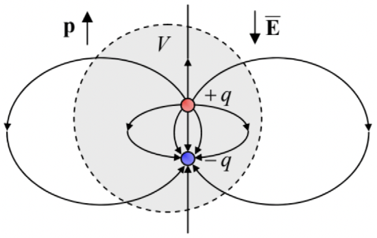Fig. 3.3. A sketch illustrating the origin of Eq. (24).

In order to be used as a reasonable coarse-grain model, Eq. (13) may be modified as follows:

\[\ \mathbf{E}_{\mathrm{cg}}=\frac{1}{4 \pi \varepsilon_{0}}\left[\frac{3 \mathbf{r}(\mathbf{r} \cdot \mathbf{p})-\mathbf{p} r^{2}}{r^{5}}-\frac{4 \pi}{3} \mathbf{p} \delta(\mathbf{r})\right],\tag{3.25}\]

so that its average satisfies Eq. (24). Evidently, such a modification does not change the field at large distances \(\ r >> a\), i.e. in the region where the expansion (3), and hence Eq. (13), are valid.

---

Reference

¹ See, e.g., MA Eq. (2.11b).

² See, e.g., MA Eq. (10.8) with \(\ \partial / \partial \varphi=0\).

³ This force is calculated, using several models, in the QM and SM parts of this series.

⁴ The equivalence may be proved, for example, by using MA Eq. (11.6) with \(\ \mathbf{f}=\mathbf{p}=\text { const }\) and \(\ \mathbf{g}=\mathbf{E}_{\text {ext }}\), taking into account that according to the general Eq. (1.28), \(\ \nabla \times \mathbf{E}_{\text {ext }}=0\).

⁵ See, e.g., the end of Sec. 4.1 in the textbook by J. Jackson, Classical Electrodynamics, 3^rd ed., Wiley, 1999.