3.2: Dipole Media

Let us generalize Eq. (7) to the case of several (possibly, many) dipoles \(\ \mathbf{p}_{j}\) located at arbitrary points \(\ \mathbf{r}_{j}\). Using the linear superposition principle, we get

\[\ \phi_{\mathrm{d}}(\mathbf{r})=\frac{1}{4 \pi \varepsilon_{0}} \sum_{j} \mathbf{p}_{j} \cdot \frac{\mathbf{r}-\mathbf{r}_{j}}{\left|\mathbf{r}-\mathbf{r}_{j}\right|^{3}}.\tag{3.26}\]

If our system (medium) contains many similar dipoles, distributed in space with density \(\ n(\mathbf{r})\), we may approximate the last sum with a macroscopic potential, which is the average of the “microscopic” potential (26) over a local volume much larger than the distance between the dipoles, and as a result, is given by the integral

\[\ \phi_{\mathrm{d}}(\mathbf{r})=\frac{1}{4 \pi \varepsilon_{0}} \int \mathbf{P}\left(\mathbf{r}^{\prime}\right) \cdot \frac{\mathbf{r}-\mathbf{r}^{\prime}}{\left|\mathbf{r}-\mathbf{r}^{\prime}\right|^{3}} d^{3} r^{\prime}, \quad \text { with } \mathbf{P}(\mathbf{r}) \equiv n(\mathbf{r}) \mathbf{p},\tag{3.27}\]

where the vector \(\ \mathbf{P}(\mathbf{r})\), called the electric polarization, has the physical meaning of the net dipole moment per unit volume. (Note that by its definition, \(\ \mathbf{P}(\mathbf{r})\) is also a “macroscopic” field.)

Now comes a very impressive trick, which is the basis of all the theory of “macroscopic” electrostatics (and eventually, “macroscopic” electrodynamics). Just as was done at the derivation of Eq. (5), Eq. (27) may be rewritten in the equivalent form

\[\ \phi_{\mathrm{d}}(\mathbf{r})=\frac{1}{4 \pi \varepsilon_{0}} \int \mathbf{P}\left(\mathbf{r}^{\prime}\right) \cdot \nabla^{\prime} \frac{1}{\left|\mathbf{r}-\mathbf{r}^{\prime}\right|} d^{3} r^{\prime},\tag{3.28}\]

where \(\ \nabla^{\prime}\) means the del operator (in this particular case, the gradient) acting in the “source space” of vectors \(\ \mathbf{r}^{\prime}\). The right-hand side of Eq. (28), applied to any volume \(\ V\) limited by surface \(\ S\), may be integrated by parts to give⁶

\[\ \phi_{\mathrm{d}}(\mathbf{r})=\frac{1}{4 \pi \varepsilon_{0}} \oint_{S} \frac{P_{n}\left(\mathbf{r}^{\prime}\right)}{\left|\mathbf{r}-\mathbf{r}^{\prime}\right|} d^{2} r^{\prime}-\frac{1}{4 \pi \varepsilon_{0}} \int_{V} \frac{\nabla^{\prime} \cdot \mathbf{P}\left(\mathbf{r}^{\prime}\right)}{\left|\mathbf{r}-\mathbf{r}^{\prime}\right|} d^{3} r^{\prime}.\tag{3.29}\]

If the surface does not carry an infinitely dense (\(\ \delta\)-functional) sheet of additional dipoles, or it is just very distant, the first term on the right-hand side is negligible.⁷ Now comparing the second term with the basic equation (1.38) for the electric potential, we see that this term may be interpreted as the field of certain effective electric charges with density

Effective charge density

\[\ \rho_{\mathrm{ef}}=-\nabla \cdot \mathbf{P}.\tag{3.30}\]

Figure 4 illustrates the physics of this key relation for a cartoon model of a simple multi-dipole system: a layer of uniformly-distributed two-point-charge units oriented perpendicular to the layer surface. (In this case \(\ \nabla \cdot \mathbf{P}=d P / d x\).) One can see that the \(\ \rho_{\mathrm{ef}}\) defined by Eq. (30) may be interpreted as the density of the uncompensated surface charges of polarized elementary dipoles.

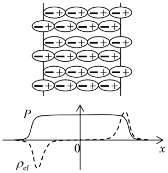Fig. 3.4. The spatial distributions of the polarization and effective charges in a layer of similar elementary dipoles (schematically).

Next, from Sec. 1.2, we already know that Eq. (1.38) is equivalent to the inhomogeneous Maxwell equation (1.27) for the electric field, so that the macroscopic electric field of the dipoles (defined as \(\ \mathbf{E}_{\mathrm{d}}=-\nabla \phi_{\mathrm{d}}\), where \(\ \phi_{\mathrm{d}}\) is given by Eq. (27)) obeys a similar equation, with the effective charge density (30).

Now let us consider a more general case when a system, besides the compensated charges of the dipoles, also has certain stand-alone charges (not parts of the dipoles already taken into account in the polarization \(\ \mathbf{P}\)). As was discussed in Sec. 1.1, if we average this charge over the inter-point-charge
distances, i.e. approximate it with a continuous “macroscopic” density \(\ \rho(\mathbf{r})\), then its macroscopic electric field also obeys Eq. (1.27), but with the stand-alone charge density. Due to the linear superposition principle, for the total macroscopic field \(\ \mathbf{E}\) of these charges and dipoles, we may write

\[\ \nabla \cdot \mathbf{E}=\frac{1}{\varepsilon_{0}}\left(\rho+\rho_{\mathrm{ef}}\right)=\frac{1}{\varepsilon_{0}}(\rho-\nabla \cdot \mathbf{P})\tag{3.31}\]

This is already the main result of the “macroscopic” electrostatics. However, it is evidently tempting (and very convenient for applications) to rewrite Eq. (31) in a different form by carrying the dipole-related term of this equality over to its left-hand side. The resulting formula is called the macroscopic Maxwell equation for D:

Maxwell equation for D

\[\ \nabla \cdot \mathbf{D}=\rho,\tag{3.32}\]

where \(\ \mathbf{D}(\mathbf{r})\) is a new “macroscopic” field, called the electric displacement, defined as⁸

Electric displacement

\[\ \mathbf{D} \equiv \varepsilon_{0} \mathbf{E}+\mathbf{P}.\tag{3.33}\]

The comparison of Eqs. (32) and (1.27) shows that \(\ \mathbf{D}\) (or more strictly, the fraction \(\ \left.\mathbf{D} / \varepsilon_{0}\right)\)) may be interpreted as the “would-be” electric field that would be created by stand-alone charges in the absence of the dipole medium polarization. In contrast, the \(\ \mathbf{E}\) participating in Eqs. (31) and (33) is the genuine (if macroscopic) electric field, exact at distances much larger than that between the adjacent elementary charges and dipoles.

In order to get an even better gut feeling of the fields \(\ \mathbf{E}\) and \(\ \mathbf{D}\), let us first rewrite the macroscopic Maxwell equation (32) in the integral form. Applying the divergence theorem to an arbitrary volume \(\ V\) limited by surface \(\ S\), we get the following macroscopic Gauss law:

Macroscopic Gauss law

\[\ \oint_{S} D_{n} d^{2} r=\int_{V} \rho d^{3} r \equiv Q,\tag{3.34}\]

where \(\ Q\) is the stand-alone charge inside volume \(\ V\).

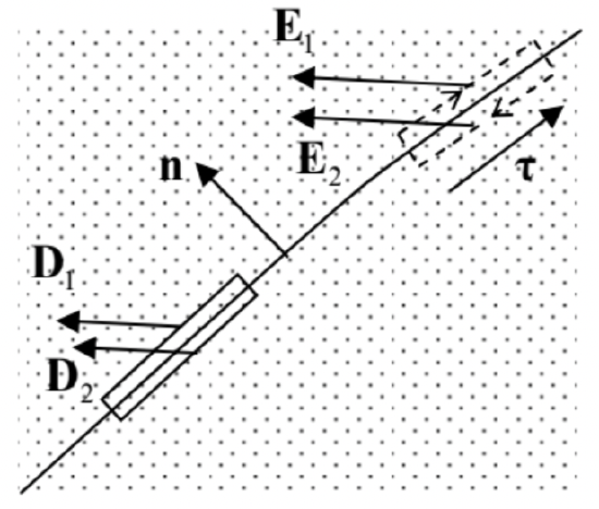
This general result may be used to find the boundary conditions for \(\ \mathbf { D }\) at a sharp interface between two different dielectrics. (The analysis is applicable to a dielectric/free-space boundary as well.) For that, let us apply Eq. (34) to a flat pillbox formed at the interface (see the solid rectangle in Fig. 5), which is sufficiently small on the spatial scales of the dielectric’s nonuniformity and the interface’s curvature, but still containing many elementary dipoles. Assuming that the interface does not have stand-alone surface charges, we immediately get

Boundary condition for D

\[\ \left(D_{n}\right)_{1}=\left(D_{n}\right)_{2},\tag{3.35}\]

i.e. the normal component of the electric displacement has to be continuous. Note that a similar statement for the macroscopic electric field \(\ \mathbf{E}\) is generally not valid, because the polarization vector \(\ \mathbf{ P }\) may have, and typically does have a leap at a sharp interface (say, due to the different polarizability of the two different dielectrics), providing a surface layer of the effective charges (30) – see again the example shown in Fig. 4.

Fig. 3.5. Deriving the boundary conditions at an interface between two dielectrics, using a Gauss pillbox (shown as a solid-line rectangle) and a circulation contour (dashed- line rectangle). \(\ \mathbf{n}\) and \(\ \boldsymbol{\tau}\) are the unit vectors, which are, respectively, normal and tangential to the interface.

However, we still can make an important statement about the behavior of \(\ \mathbf{E}\) at the interface. Indeed, the macroscopic electric fields defined by Eqs. (29) and (31), are evidently still potential ones, and hence obey the macroscopic Maxwell equation, similar to Eq. (1.28):

Macroscopic Maxwell equation for E

\[\ \nabla \times \mathbf{E}=0.\tag{3.36}\]

Integrating this equality along a narrow contour stretched along the interface (see the dashed rectangle in Fig. 5), we get

Boundary condition for E

\[\ \left(E_{\tau}\right)_{1}=\left(E_{\tau}\right)_{2}.\tag{3.37}\]

Note that this condition is compatible with (and may be derived from) the continuity of the macroscopic electrostatic potential \(\ \phi\) (related to the macroscopic field \(\ \mathbf{E}\) by the relation similar to Eq. (1.33), \(\ \mathbf{E}=-\nabla \phi\)), at each point of the interface: \(\ \phi_{1}=\phi_{2}\).

In order to see how these boundary conditions work, let us consider the simple problem shown in Fig. 6. A very broad plane capacitor, with zero voltage between its conducting plates (as may be enforced, for example, by their connection with an external wire), is partly filled with a material with a uniform polarization \(\ \mathbf{P}_{0}\),⁹ oriented normal to the plates. Let us calculate the spatial distribution of the fields \(\ \mathbf{E}\) and \(\ \mathbf { D }\), and also the surface charge density of each conducting plate.

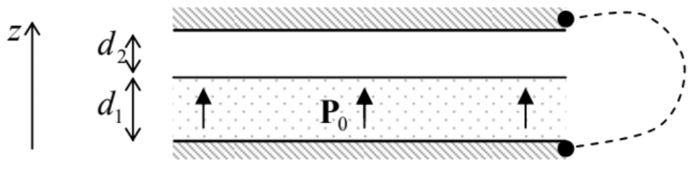Fig. 3.6. A simple system whose analysis requires Eq. (35).

Due to the symmetry of the system, the vectors \(\ \mathbf{E}\) and \(\ \mathbf { D }\) are both normal to the plates and do not depend on the position in the capacitor’s plane, so that we can limit the field analysis to the calculation of their \(\ z\)-components \(\ E(z)\) and \(\ D(z)\). In this case, the Maxwell equation (32) is reduced to \(\ d D / d z=0\) inside each layer (but not at their border!), so that within each of them, \(\ D\) is constant – say, some \(\ D_{1}\) in the layer with \(\ \mathbf{P}=\mathbf{P}_{0}\), and certain \(\ D_{2}\) in the free-space layer, where \(\ \mathbf{P}=0\). As a result, according to Eq. (33), the (macroscopic) electric field inside each layer in also constant:

\[\ D_{1}=\varepsilon_{0} E_{1}+P_{0}, \quad D_{2}=\varepsilon_{0} E_{2}.\tag{3.38}\]

Since the voltage between the plates is zero, we may also require the integral of \(\ E\), taken along a path connecting the plates, to vanish. This gives us one more relation:

\[\ E_{1} d_{1}+E_{2} d_{2}=0.\tag{3.39}\]

Still, three equations (38)-(39) are insufficient to calculate the four fields in the system (\(\ E_{1,2}\) and \(\ D_{1,2}\)). The decisive help comes from the boundary condition (35):

\[\ D_{1}=D_{2}.\tag{3.40}\]

(Note that it is valid because the layer interface does not carry stand-alone electric charges, even though it has a polarization surface charge, whose areal density may be calculated by integrating Eq. (30) across the interface: \(\ \sigma_{\mathrm{ef}}=P_{0}\). Note also that in our simple system, Eq. (37) is identically satisfied due to
the system’s symmetry, and hence does not give any additional information.)

Now solving the resulting system of four equations (38)-(40), we readily get

\[\ E_{1}=-\frac{P_{0}}{\varepsilon_{0}} \frac{d_{2}}{d_{1}+d_{2}}, \quad E_{2}=\frac{P_{0}}{\varepsilon_{0}} \frac{d_{1}}{d_{1}+d_{2}}, \quad D_{1}=D_{2}=D=P_{0} \frac{d_{1}}{d_{1}+d_{2}}.\tag{3.41}\]

The areal densities of the electrode surface charges may now be readily calculated by the integration of Eq. (32) across each surface:

\[\ \sigma_{1}=-\sigma_{2}=D=P_{0} \frac{d_{1}}{d_{1}+d_{2}}.\tag{3.42}\]

Note that due to the spontaneous polarization of the lower layer’s material, the capacitor plates are charged even in the absence of voltage between them, and that this charge is a function of the second electrode’s position \(\ \left(d_{2}\right)\).¹⁰ Also notice substantial similarity between this system (Fig. 6), and the one
whose analysis was the subject of Problem 2.6.

---

Reference

⁶ To prove this (almost evident) formula strictly, it is sufficient to apply the divergence theorem given by MA Eq. (12.2), to the vector function \(\ \mathbf{f}=\mathbf{P}\left(\mathbf{r}^{\prime}\right) /\left|\mathbf{r}-\mathbf{r}^{\prime}\right|\), in the “source space” of radius-vectors \(\ \mathbf{r}^{\prime}\).

⁷ Just like in the case of Eq. (1.9), we may always describe such a dipole sheet using the second term in Eq. (29), by including a delta-functional part into the polarization distribution \(\ \mathbf{P}\left(\mathbf{r}^{\prime}\right)\).

⁸ Note that according to its definition (33), the dimensionality of \(\ \mathbf { D }\) in the SI units is different from that of \(\ \mathbf{E}\). In contrast, in the Gaussian units the electric displacement is defined as \(\ \mathbf{D}=\mathbf{E}+4 \pi \mathbf{P}\), so that \(\ \nabla \cdot \mathbf{D}=4 \pi \rho\) (the relation \(\ \rho_{\mathrm{ef}}=-\nabla \cdot \mathbf{P}\) remains the same as in SI units), and the dimensionalities of \(\ \mathbf { D }\) and \(\ \mathbf{E}\) coincide. This coincidence is a certain perceptional handicap because it is frequently convenient to consider the scalar components of \(\ \mathbf{E}\) as generalized forces, and those of \(\ \mathbf { D }\) as generalized coordinates (see Sec. 5 below), and it is somewhat comforting to have their dimensionalities different, as they are in the SI units.

⁹ As will be discussed in the next section, this is a good approximation for the so-called electrets, and also for hard ferroelectrics in not very high electric fields.

¹⁰ This effect is used in most modern microphones. In such a device, the sensed sound wave’s pressure bends a thin conducting membrane playing the role of one of the capacitor’s plates, and thus modulates the thickness (in Fig. 6, \(\ d_{2}\)) of the air gap adjacent to the electret layer. This modulation produces proportional variations of the charges (42), and hence some electric current in the wire connecting the plates, which is picked up by readout electronics.