7.3: Reflection

The most important new effect arising in nonuniform media is wave reflection. Let us start its discussion from the simplest case of a plane electromagnetic wave that is normally incident on a sharp interface between two uniform, linear, isotropic media.

Let us start with the simplest case when one of the two media (say, that located at \(\ z>0\), see Fig. 8) cannot sustain any electric field at all – as implied, in particular, by the macroscopic model of a good conductor – see Eq. (2.1):

\[\ \left.E\right|_{z \geq 0}=0.\tag{7.57}\]

This condition is evidently incompatible with the single traveling wave (5). However, this solution may be readily corrected using the fact that the dispersion-free 1D wave equation,

\[\ \left(\frac{\partial^{2}}{\partial z^{2}}-\frac{1}{\nu^{2}} \frac{\partial^{2}}{\partial t^{2}}\right) E=0,\tag{7.58}\]

supports waves propagating, with the same speed, in opposite directions. As a result, the following linear superposition of two such waves,

\[\ \left.E\right|_{z \leq 0}=f(z-\nu t)-f(-z-\nu t),\tag{7.59}\]

satisfies both the equation and the boundary condition (57), for an arbitrary function \(\ f\). The second term in Eq. (59) may be interpreted as a result of total reflection of the incident wave (described by its first term) – in this particular case, with the change of the electric field’s sign. This means, in particular, that within the macroscopic model, a conductor acts as a perfect mirror. By the way, since the vector n of the reflected wave is opposite to that incident one (see the arrows in Fig. 8), Eq. (6) shows that the magnetic field of the wave does not change its sign at the reflection:

\[\ \left.H\right|_{z \leq 0}=\frac{1}{Z}[f(z-\nu t)+f(-z-\nu t)]\tag{7.60}\]

Fig. 7.8. A snapshot of the electric field at the reflection of a sinusoidal wave from a perfect conductor: a realistic pattern (red lines) and its macroscopic, ideal-mirror approximation (blue lines). Dashed lines show the snapshots after a half-period time delay \(\ (\omega \Delta t=\pi)\).

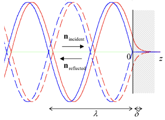
The blue lines in Fig. 8 show the resulting pattern (59) for the simplest, monochromatic wave:

\[\ \text{Wave’s total reflection}\quad\quad\quad\quad \left.E\right|_{z \leq 0}=\operatorname{Re}\left[E_{\omega} e^{i(k z-\omega t)}-E_{\omega} e^{i(-k z-\omega t)}\right].\tag{7.61a}\]

Depending on convenience in a particular context, this pattern may be legitimately represented and interpreted either as the linear superposition (61a) of two traveling waves or as a single standing wave:

\[\ \left.E\right|_{z \leq 0}=-2 \operatorname{Im}\left(E_{\omega} e^{-i \omega t}\right) \sin k z \equiv 2 \operatorname{Re}\left(i E_{\omega} e^{-i \omega t}\right) \sin k z \equiv 2 \operatorname{Re}\left[E_{\omega} e^{-i(\omega t-\pi / 2)}\right] \sin k z,\tag{7.61b}\]

in which the electric and magnetic field oscillate with the phase shifts by \(\ \pi / 2\) both in time and space:

\[\ \left.H\right|_{z \leq 0}=\operatorname{Re}\left[\frac{E_{\omega}}{Z} e^{i(k z-\omega t)}+\frac{E_{\omega}}{Z} e^{i(-k z-\omega t)}\right] \equiv 2 \operatorname{Re}\left(\frac{E_{\omega}}{Z} e^{-i \omega t}\right) \cos k z.\tag{7.62}\]

As a result of this shift, the time average of the Poynting vector’s magnitude,

\[\ S(z, t)=E H=\frac{1}{Z} \operatorname{Re}\left[E_{\omega}^{2} e^{-2 i \omega t}\right] \sin 2 k z,\tag{7.63}\]

equals zero, showing that at the total reflection there is no average power flow. (This is natural because the perfect mirror can neither transmit the wave nor absorb it.) However, Eq. (63) shows that the standing wave provides local oscillations of energy, transferring it periodically between the concentrations of the electric and magnetic fields, separated by the distance \(\ \Delta z=\pi / 2 k=\lambda / 4\).

In the case of the sinusoidal waves, the reflection effects may be readily explored even for the more general case of dispersive and/or lossy (but still linear) media in which \(\ \varepsilon(\omega)\) and \(\ \mu(\omega)\), and hence the wave vector \(\ k(\omega)\) and the wave impedance \(\ Z(\omega)\), defined by Eqs. (28), are certain complex functions of frequency. The “only” new factors we have to account for is that in this case, the reflection may not be total, and that inside the second media we have to use the traveling-wave solution as well. Both these factors may be taken care of by looking for the solution to our boundary problem in the form

\[\ \left.E\right|_{z \leq 0}=\operatorname{Re}\left[E_{\omega}\left(e^{i k_{-} z}+R e^{-i k_{-} z}\right) e^{-i \omega t}\right],\left.\quad E\right|_{z \geq 0}=\operatorname{Re}\left[E_{\omega} T e^{i k_{+} z} e^{-i \omega t}\right],\quad\quad\quad\quad \text{Wave’s partial reflection}\tag{7.64}\]

and hence, according to Eq. (6),

\[\ \left.H\right|_{z \leq 0}=\operatorname{Re}\left[\frac{E_{\omega}}{Z_{-}(\omega)}\left(e^{i k_{-} z}-R e^{-i k_{-} z}\right) e^{-i \omega t}\right],\left.\quad H\right|_{z \geq 0}=\operatorname{Re}\left[\frac{E_{\omega}}{Z_{+}(\omega)} T e^{i k_{+} z} e^{-i \omega t}\right].\tag{7.65}\]

(The indices + and – correspond to the media located at \(\ z>0\) and \(\ z<0\), respectively.) Please note the following important features of these solutions:

(i) Due to the problem’s linearity, we could (and did :-) take the complex amplitudes of the reflected and transmitted wave proportional to that \(\ \left(E_{\omega}\right)\) of the incident wave, while scaling them with dimensionless, generally complex coefficients \(\ R\) and \(\ T\). As the comparison of Eqs. (64)-(65) with Eqs. (61)-(62) shows, the total reflection from an ideal mirror that was discussed above, corresponds to the particular case \(\ R=-1\) and \(\ T=0\).

(ii) Since the incident wave that we are considering, arrives from one side only (from \(\ z=-\infty\)), there is no need to include a term proportional to \(\ \exp \left\{-i k_{+} z\right\}\) into Eqs. (64)-(65) – in our current problem. However, we would need such a term if the medium at \(\ z>0\) had been nonuniform (e.g., had at least one more interface or any other inhomogeneity), because the wave reflected from that additional inhomogeneity would be incident on our interface (located at \(\ z=0\)) from the right.

(iii) The solution (64)-(65) is sufficient even for the description of the cases when waves cannot propagate to \(\ z \geq 0\), for example a conductor or a plasma with \(\ \omega_{\mathrm{p}}>\omega\). Indeed, the exponential drop of the field amplitude at \(\ z>0\) in such cases is automatically described by the imaginary part of the wave
number \(\ k_{+}\) – see Eq. (29).

In order to calculate the coefficients \(\ R\) and \(\ T\), we need to use boundary conditions at \(\ z=0\). Since the reflection does not change the transverse character of the partial waves, in our current case of the normal incidence, both vectors E and H remain tangential to the interface plane (in our notation, \(\ z = 0\)).

Reviewing the arguments that have led us, in statics, to the boundary conditions (3.37) and (5.117) for these components, we see that they remain valid for the time dependent situation as well,²⁷ so that for our current case of normal incidence we may write:

\[\ \left.E\right|_{z=-0}=\left.E\right|_{z=+0},\left.\quad H\right|_{z=-0}=\left.H\right|_{z=+0}.\tag{7.66}\]

Plugging Eqs. (64)-(65) into these conditions, we readily get two equations for the coefficients \(\ R\) and \(\ T\):

\[\ 1+R=T, \quad \frac{1}{Z_{-}}(1-R)=\frac{1}{Z_{+}} T.\tag{7.67}\]

Solving this simple system of linear equations, we get²⁸

\[\ \text{Reflection and transmission: sharp interface}\quad\quad\quad\quad R=\frac{Z_{+}-Z_{-}}{Z_{+}+Z_{-}}, \quad T=\frac{2 Z_{+}}{Z_{+}+Z_{-}}.\tag{7.68}\]

These formulas are very important, and much more general than one might think because they are applicable for virtually any 1D waves – electromagnetic or not, provided that the impedance \(\ Z\) is defined properly.²⁹ Since in the general case the wave impedances \(\ Z_{\pm}\) defined by Eq. (28) with the corresponding indices, are complex functions of frequency, Eqs. (68) show that \(\ R\) and \(\ T\) may have imaginary parts as well. This fact has important consequences at \(\ z<0\), where the reflected wave,
proportional to \(\ R\), combines (“interferes”) with the incident wave. Indeed, with \(\ R=|R| e^{i \varphi}\) (where \(\ \varphi \equiv\) arg \(\ R\) is a real phase shift), the expression in the parentheses in the first of Eqs. (64) becomes

\[\ \begin{aligned}
e^{i k_{-} z}+R e^{-i k_{-} z} &=(1-|R|+|R|) e^{i k_{-} z}+|R| e^{i \varphi} e^{-i k_{-} z} \\
& \equiv(1-|R|) e^{i k_{-} z}+2|R| e^{i \varphi / 2} \sin \left[k_{-}\left(z-\delta_{-}\right)\right], \quad \text { where } \delta_{-} \equiv \frac{\varphi-\pi}{2 k_{-}} .
\end{aligned}\tag{7.69}\]

This means that the field may be represented as a sum of a traveling wave and a standing wave, with an amplitude proportional to \(\ |R|\), shifted by the distance \(\ \delta_{-}\) toward the interface, relatively to the ideal-mirror pattern (61b) – see Fig. 8. This effect is frequently used for the experimental measurements of an unknown impedance \(\ Z_{+}\) of some medium, provided than \(\ Z_{-}\) is known – most often, the free space, where \(\ Z_{-}=Z_{0}\). For that, a small antenna (the probe), not disturbing the fields’ distribution too much, is placed into the wave field, and the amplitude of the ac voltage induced in it by the wave in the probe is measured with a detector (e.g., a semiconductor diode with a nearly-quadratic I-V curve), as a function of \(\ z\) (Fig. 9). From the results of such a measurement, it is straightforward to find both \(\ |R|\) and \(\ \delta\_\), and hence restore the complex \(\ R\), and then use Eq. (67) to calculate both the modulus and the argument of \(\ Z_{+}\). (Before computers became ubiquitous, a specially lined paper called the Smith chart, had been frequently used for performing this recalculation graphically; it is still used for result presentation.)

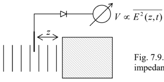Fig. 7.9. Measurement of the complex impedance of a medium (schematically).

Now let us discuss what do these results give for waves incident from the free space \(\ \left(Z_{-}(\omega)=Z_{0}\right.=\text{const}\), \(\ k_{-}=k_{0}=\omega / c\)) onto the surfaces of two particular, important media.

(i) For a collision-free plasma (with negligible magnetization) we may use Eq. (36) with \(\ \mu(\omega)=\mu_0\), to represent the impedance (28) in either of two equivalent forms:

\[\ Z_{+}=Z_{0} \frac{\omega}{\left(\omega^{2}-\omega_{\mathrm{p}}^{2}\right)^{1 / 2}} \equiv-i Z_{0} \frac{\omega}{\left(\omega_{\mathrm{p}}^{2}-\omega^{2}\right)^{1 / 2}}.\tag{7.70}\]

The first of these forms is more convenient in the case \(\ \omega>\omega_{\mathrm{p}}\), when the wave vector \(\ k_{+}\) and the wave impedance \(\ Z_{+}\) of plasma are real, so that a part of the incident wave does propagate into the plasma. Plugging this expression into the latter of Eqs. (68), we see that \(\ T\) is real as well:

\[\ T=\frac{2 \omega}{\omega+\left(\omega^{2}-\omega_{\mathrm{p}}^{2}\right)^{1 / 2}}.\tag{7.71}\]

Note that according to this formula, and somewhat counter-intuitively, \(\ T>1\) for any frequency (above \(\ \omega_{\mathrm{p}}\)), inviting the question: how can the transmitted wave be more intensive than the incident one that has induced it? For answering this question, we need to compare the powers (rather than the electric field amplitudes) of these two waves, i.e. their average Poynting vectors (42):

\[\ \overline{S_{\text {incident }}}=\frac{\left|E_{\omega}\right|^{2}}{2 Z_{0}}, \quad \overline{S_{+}}=\frac{\left|T E_{\omega}\right|^{2}}{2 Z_{+}}=\frac{\left|E_{\omega}\right|^{2}}{2 Z_{0}} \frac{4 \omega\left(\omega^{2}-\omega_{\mathrm{p}}^{2}\right)^{1 / 2}}{\left[\omega+\left(\omega^{2}-\omega_{\mathrm{p}}^{2}\right)^{1 / 2}\right]^{2}}.\tag{7.72}\]

The ratio of these two values³⁰ is always below 1 (and tends to zero at \(\ \omega \rightarrow \omega_{\mathrm{p}}\)), so that only a fraction of the incident wave power may be transmitted. Hence the result \(\ T>1\) may be interpreted as follows: an interface between two media may be an impedance transformer: it can never transmit more power than the incident wave provides, i.e. can only decrease the product \(\ S=E H\), but since the ratio \(\ Z=E / H\) changes at the interface, the amplitude of one of the fields may increase at the transmission.

Now let us proceed to case \(\ \omega<\omega_{\mathrm{p}}\), when the waves cannot propagate in the plasma. In this case, the second of the expressions (70) is more convenient, because it immediately shows that \(\ Z_{+}\) is purely imaginary, while \(\ Z_{-}=Z_{0}\) is purely real. This means that \(\ \left(Z_{+-} Z_{-}\right)=\left(Z_{+}+Z_{-}\right)^{*}\), i.e. according to the first of Eqs. (68), \(\ |R|=1\), so that the reflection is total, i.e. no incident power (on average) is transferred into
the plasma – as was already discussed in Sec. 2. However, the complex \(\ R\) has a finite argument,

\[\ \varphi \equiv \arg R=2 \arg \left(Z_{+}-Z_{0}\right)=-2 \tan ^{-1} \frac{\omega}{\left(\omega_{\mathrm{p}}^{2}-\omega^{2}\right)^{1 / 2}},\tag{7.73}\]

and hence provides a finite spatial shift (69) of the standing wave toward the plasma surface:

\[\ \delta_{-}=\frac{\varphi-\pi}{2 k_{0}}=\frac{c}{\omega} \tan ^{-1} \frac{\omega}{\left(\omega_{\mathrm{p}}^{2}-\omega^{2}\right)^{1 / 2}}.\tag{7.74}\]

On the other hand, we already know from Eq. (40) that the solution at \(\ z>0\) is exponential, with the decay length \(\ \delta\) that is described by Eq. (39). Calculating, from the coefficient \(\ T\), the exact coefficient before this exponent, it is straightforward to verify that the electric and magnetic fields are indeed continuous at the interface, completing the pattern shown with red lines in Fig. 8. This wave penetration into a fully reflecting material may be experimentally observed, for example, by thinning its sample. Even without solving this problem exactly, it is evident that if the sample thickness d becomes comparable to \(\ \delta\), a part of the exponential “tail” of the field reaches the second interface, and induces a propagating wave. This is a classical electromagnetic analog of the quantum-mechanical tunneling through a potential barrier.³¹

Note that at low frequencies, both \(\ \delta\_\) and \(\ \delta\) tend to the same frequency-independent value,

\[\ \delta, \delta_{-} \rightarrow \frac{c}{\omega_{\mathrm{p}}}=\left(\frac{c^{2} \varepsilon_{0} m_{\mathrm{e}}}{n e^{2}}\right)^{1 / 2}=\left(\frac{m_{\mathrm{e}}}{\mu_{0} n e^{2}}\right)^{1 / 2}, \quad \text { at } \frac{\omega}{\omega_{\mathrm{p}}} \rightarrow 0,\tag{7.75}\]

which is just the field penetration depth (6.44) calculated for a perfect conductor model (assuming \(\ m=m_{\mathrm{e}}\) and \(\ \mu=\mu_{0}\)) in the quasistatic limit. This is natural, because the condition \(\ \omega<<\omega_{\mathrm{p}}\) may be recast as \(\ \lambda_0\equiv 2 \pi c / \omega>>2 \pi c / \omega_{\mathrm{p}} \equiv 2 \pi \delta\), i.e. as the quasistatic approximation’s validity condition.

(ii) Now let us consider electromagnetic wave reflection from an Ohmic, non-magnetic conductor. In the simplest low-frequency limit, when \(\ \omega \tau\), is much less than 1, the conductor may be described by a frequency-independent conductivity \(\ \sigma\).³² According to Eq. (46), in this case we can take

\[\ Z_{+}=\left(\frac{\mu_{0}}{\varepsilon_{\mathrm{opt}}(\omega)+i \sigma / \omega}\right)^{1 / 2}.\tag{7.76}\]

With this substitution, Eqs. (68) immediately give us all the results of interest. In particular, in the most important quasistatic limit (when \(\ \delta_{\mathrm{s}} \equiv\left(2 / \mu_{0} \sigma \omega\right)^{1 / 2}<<\lambda_{0} \equiv 2 \pi c / \omega\), i.e. \(\ \sigma / \omega>>\varepsilon_{0} \sim \varepsilon_{\mathrm{opt}}\), the conductor’ impedance is low:

\[\ Z_{+} \approx\left(\frac{\mu_{0} \omega}{i \sigma}\right)^{1 / 2} \equiv \pi\left(\frac{2}{i}\right)^{1 / 2} \frac{\delta_{s}}{\lambda_{0}} Z_{0}, \quad \text { i.e. }\left|\frac{Z_{+}}{Z_{0}}\right|<<1.\tag{7.77}\]

This impedance is complex, and hence some fraction \(\ \mathscr{F}\) of the incident wave is absorbed by the conductor. The fraction may be found as the ratio of the dissipated power (either calculated, as was done above, from Eqs. (68), or just taken from Eq. (6.36), with the magnetic field amplitude \(\ \left|H_{\omega}\right|=2\left|E_{\omega}\right| / Z_{0}\) - see Eq. (62)) to the incident wave’s power given by the first of Eqs. (72). The result,

\[\ \mathscr{F}=\frac{2 \omega \delta_{s}}{c} \equiv 4 \pi \frac{\delta_{\mathrm{s}}}{\lambda_{0}}<<1.\tag{7.78}\]

is widely used for crude estimates of the energy dissipation in metallic-wall waveguides and resonators. It shows that to keep the energy losses low, the characteristic size of such systems (which gives a scale of the free-space wavelengths \(\ \lambda_{0}\) at which they are used) should be much larger than \(\ \delta_{\mathrm{s}}\). A more detailed theory of these structures, and the effects of energy loss in them, will be discussed later in this chapter.

---

Reference

²⁷ For example, the first of conditions (66) may be obtained by integrating the full (time-dependent) Maxwell equation \(\ \boldsymbol{\nabla} \times \mathbf{E}+\partial \mathbf{B} / \partial t=0\) over a narrow and long rectangular contour with dimensions \(\ l\) and \(\ d(d<<l)\) stretched along the interface. At the application of the Stokes theorem to this integral, the first term gives \(\ \Delta E_{\tau} l\), while the contribution of the second term is proportional to the product \(\ dl\), so that its contribution at \(\ d / l \rightarrow 0\) is negligible. The proof of the second boundary condition is similar – as was already discussed in Sec. 6.2.

²⁸ Please note that only the media impedances (rather than wave velocities) are important for the reflection in this case! Unfortunately, this fact is not clearly emphasized in some textbooks that discuss only the case \(\ \mu_{\pm}=\mu_{0}\), when \(\ Z=\left(\mu_{0} / \varepsilon\right)^{1 / 2}\) and \(\ \nu=1 /\left(\mu_{0} \varepsilon\right)^{1 / 2}\) are proportional to each other.

²⁹ See, e.g., the discussion of elastic waves of mechanical deformation in CM Secs. 6.3, 6.4, 7.7, and 7.8.

³⁰ This ratio is sometimes also called the “transmission coefficient”, but to avoid its confusion with the T defined by Eq. (64), it is better to call it the power transmission coefficient.

³¹ See, e.g., QM Sec. 2.3.

³² In a typical metal, \(\ \tau \sim 10^{-13} \mathrm{~s}\), so that this approximation works well up to \(\ \omega \sim 10^{13} \mathrm{~s}^{-1}\), i.e. up to the far-infrared frequencies.