
7.4: Refraction


- Last updated
- Mar 5, 2022
- Save as PDF

( \newcommand{\kernel}{\mathrm{null}\,}\)
Now let us consider the effects arising at a plane interface between two uniform media if the wave’s incidence angle θ (Fig. 10) is arbitrary, rather than equal to zero as in our previous analysis, for the simplest case of fully transparent media, with real ε±(ω) and μ±(ω). (For the sake of notation simplicity, the argument of these functions will be dropped, i.e. just implied in most formulas below.)
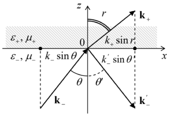
In contrast with the case of normal incidence, here the wave vectors k−,k′−, and k+ of the three components (incident, reflected, and transmitted) waves may have different directions. (Such change of the transmitted wave’s direction is called refraction.) Hence let us start our analysis with writing a general expression for a single plane, monochromatic wave for the case when its wave vector k has all three Cartesian components, rather than one. An evident generalization of Eq. (11) for this case is
f(r,t)=Re[fωei(kxx+kyy+kzz)−ωt)]≡Re[fωei(k⋅r−ωt)].
This expression enables a ready analysis of “kinematic” relations that are independent of the media impedances. Indeed, it is sufficient to notice that to satisfy any linear, homogeneous boundary conditions at the interface ( z=0), all partial plane waves must have the same temporal and spatial dependence on this plane. Hence if we select the x−z plane so that the vector k− lies in it, then (k−)y=0, and k+ and k′− cannot have any y-component either, i.e. all three wave vectors lie in the same plane – that is selected as the plane of the drawing in Fig. 10. Moreover, due to the same reason, their x-components should be equal:
k−sinθ=k′−sinθ′=k+sinr.
From here we immediately get two well-known laws: of reflection
Reflection angleθ′=θ,
and refraction:33
Snell lawsinrsinθ=k−k+.
In this form, the laws are valid for plane waves of any nature. In optics, the Snell law (82) is frequently represented in the form
sinrsinθ=n−n+,
where n± is the index of refraction, also called the “refractive index” of the corresponding medium, defined as its wave number normalized to that of the free space (at the particular wave’s frequency):
Index of refractionn±≡k±k0≡(ε±μ±ε0μ0)1/2.
Perhaps the most famous corollary of the Snell law is that if a wave propagates from a medium with a higher index of refraction to that with a lower one (i.e. if n−>n+ in Fig. 10), for example from water to air, there is always a certain critical value θc of the incidence angle,
Critical angleθc=sin−1n+n−≡sin−1(ε+μ+ε−μ−)1/2,
at which the refraction angle r (see Fig. 10 again) reaches π/2. At a larger θ, i.e. within the range θc<θ<π/2, the boundary conditions (80) cannot be satisfied by a refracted wave with a real wave vector, so that the wave experiences the so-called total internal reflection. This effect is very important for practice, because it means that dielectric surfaces may be used as optical mirrors, in particular in optical fibers – to be discussed in more detail in Sec. 7 below. This is very fortunate for telecommunication technology, because light’s reflection from metals is rather imperfect. Indeed, according to Eq. (78), in the optical range (λ0∼0.5μm, i.e. ω∼1015 s−1), even the best conductors (with σ∼6×10⁸ S/m and hence the normal skin depth δs∼1.5 nm) provide power loss of at least a few percent at each reflection.
Note, however, that even within the range θc<θ<π/2, the field at z>0, is not identically equal to zero: it penetrates into the less dense media by a distance of the order of λ0, exponentially decaying inside it, just as it does at the normal incidence – see Fig. 8. However, at θ≠0 the penetrating field still propagates, with the wave number (80), along the interface. Such a field, exponentially dropping in one direction but still propagating as a wave in another direction, is commonly called the evanescent wave.
One more remark: just as at the normal incidence, the field’s penetration into another medium causes a phase shift of the reflected wave – see, e.g., Eq. (69) and its discussion. A new feature of this phase shift, arising at θ≠0, is that it also has a component parallel to the interface – the so-called Goos- Hänchen effect. In geometric optics, this effect leads to an image shift (relative to that its position in a perfect mirror) with components both normal and parallel to the interface.
Now let us carry out an analysis of “dynamic” relations that determine amplitudes of the refracted and reflected waves. For this, we need to write explicitly the boundary conditions at the interface (i.e. the plane z=0). Since now the electric and/or magnetic fields may have components normal to the plane, in addition to the continuity of their tangential components, which were repeatedly discussed above,
Ex,y|z=−0=Ex,y|z=+0,Hx,y|z=−0=Hx,y|z=+0,
we also need relations for the normal components. As it follows from the homogeneous macroscopic Maxwell equations (6.99b), they are also the same as in statics, i.e. Dn=const, and Bn=const, for our coordinate choice (Fig. 10) giving
ε−Ez|z=−0=ε+Ez|z=+0,μ−Hz|z=−0=μ+Hz|z=+0.
The expressions of these components via the amplitudes Eω, REω, and TEω of the incident, reflected, and transmitted waves depend on the incident wave’s polarization. For example, for a linearly-polarized wave with the electric field vector perpendicular to the plane of incidence, i.e. parallel to the interface plane, the reflected and refracted waves are similarly polarized – see Fig. 11a.
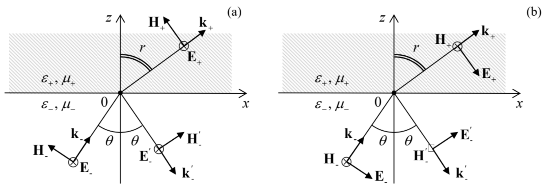 Fig. 7.11. Reflection and refraction at two different linear polarizations of the incident wave.
As a result, all Ez are equal to zero (so that the first of Eqs. (87) is inconsequential), while the tangential components of the electric field are equal to their full amplitudes, just as at the normal incidence, so we still can use Eqs. (64) expressing these components via the coefficients R and T. However, at θ≠0 the magnetic fields have not only tangential components
Hx|z=−0=Re[EωZ−(1−R)cosθe−iωt],Hx|z=+0=Re[EωZ+Tcosre−iωt],
but also normal components (see Fig. 11a):
Hz|z=−0=Re[EωZ−(1+R)sinθe−iωt],Hz|z=+0=Re[EωZ+Tsinre−iωt].
Plugging these expressions into the boundary conditions expressed by Eqs. (86) (in this case, for the y-components only) and the second of Eqs. (87), we get three equations for two unknown coefficients R and T. However, two of these equations duplicate each other because of the Snell law, and we get just two independent equations,
1+R=T,1Z−(1−R)cosθ=1Z+Tcosr,
which are a very natural generalization of Eqs. (67), with the replacements Z−→Z−cosr,Z+→Z+cosθ. As a result, we can immediately use Eq. (68) to write the solution of the system (90):34
R=Z+cosθ−Z−cosrZ+cosθ+Z−cosr,T=2Z+cosθZ+cosθ+Z−cosr.
If we want to express these coefficients via the angle of incidence alone, we should use the Snell law (82) to eliminate the angle r, getting the commonly used, more bulky expressions:
R=Z+cosθ−Z−[1−(k−/k+)2sin2θ]1/2Z+cosθ+Z−[1−(k−/k+)2sin2θ]1/2,T=2Z+cosθZ+cosθ+Z−[1−(k−/k+)2sin2θ]1/2.
However, my personal preference is to use the kinematic relation (82) and the dynamic relations (91a) separately, because Eq. (91b) obscures the very important physical fact that and the ratio of k±, i.e. of the wave velocities of the two media, is only involved in the Snell law, while the dynamic relations essentially include only the ratio of wave impedances – just as in the case of normal incidence.
In the opposite case of the linear polarization of the electric field within the plane of incidence (Fig. 11b), it is the magnetic field that does not have a normal component, so it is now the second of Eqs. (87) that does not participate in the solution. However, now the electric fields in two media have not only tangential components,
Ex|z=−0=Re[Eω(1+R)cosθe−iωt],Ex|z=+0=Re[EωTcosre−iωt],
but also normal components (Fig. 11b):
Ez|z=−0=Eω(−1+R)sinθ,Ez|z=+0=−EωTsinr.
As a result, instead of Eqs. (90), the reflection and transmission coefficients are related as
(1+R)cosθ=Tcosr,1Z−(1−R)=1Z+T.
Again, the solution of this system may be immediately written using the analogy with Eq. (67):
R=Z+cosr−Z−cosθZ+cosr+Z−cosθ,T=2Z+cosθZ+cosr+Z−cosθ,
or, alternatively, using the Snell law, in a more bulky form:
R=Z+[1−(k−/k+)2sin2θ]1/2−Z−cosθZ+[1−(k−/k+)2sin2θ]1/2+Z−cosθ,T=2Z+cosθZ+[1−(k−/k+)2sin2θ]1/2+Z−cosθ.
For the particular case μ+=μ−=μ0, when Z+/Z−=(ε−/ε+)1/2=k−/k+=n−/n+ (which is approximately correct for traditional optical media), Eqs. (91b) and (95b) are called the Fresnel formulas.35 Most textbooks are quick to point out that there is a major difference between them: while for the electric field polarization within the plane of incidence (Fig. 11b), the reflected wave’s amplitude (proportional to the coefficient R) turns to zero36 at a special value of θ (called the Brewster angle):37
θB=tan−1n+n−,
while there is no such angle in the opposite case (shown in Fig. 11a). However, note that this statement, as well as Eq. (96), is true only for the case μ+=μ−. In the general case of different ε and μ, Eqs. (91) and (95) show that the reflected wave vanishes at θ=θB with
tan2θB=ε−μ+−ε+μ−ε+μ+−ε−μ−×{(μ+/μ−),for E⊥nz (Fig.11a) (−ε+/ε−),for H⊥nz (Fig. 11b) Brewster angle
Note the natural ε↔μ symmetry of these relations, resulting from the E↔H symmetry for these two polarization cases (Fig. 11). These formulas also show that for any set of parameters of the two media (with ε±,μ±>0), tan2θB is positive (and hence a real Brewster angle θB exists) only for one of these two polarizations. In particular, if the interface is due to the change of μ alone (i.e. if ε+=ε−), the first of Eqs. (97) is reduced to the simple form (96) again, while for the polarization shown in Fig. 11b there is no Brewster angle, i.e. the reflected wave has a non-zero amplitude for any θ.
Such an account of both media parameters, ε and μ, on an equal footing is necessary to describe the so-called negative refraction effects.38 As was shown in Sec. 2, in a medium with electric-field-driven resonances, the function ε(ω) may be almost real and negative, at least within limited frequency
intervals – see, in particular, Eq. (34) and Fig. 5. As has already been discussed, if, at these frequencies, the function μ(ω) is real and positive, then k2(ω)=ω2ε(ω)μ(ω)<0, and k may be represented as i/δ with a real δ, meaning the exponential field decay into the medium. However, let us consider the case when both ε(ω)<0 and μ(ω)<0 at a certain frequency. (This is possible in a medium with both E-driven and H-driven resonances, at a proper choice of their resonance frequencies.) Since in this case k2(ω)=ω2ε(ω)μ(ω)>0, the wave vector is real, so that Eq. (79) describes a traveling wave, and one could think that there is nothing new in this case. Not so!
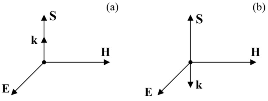
First of all, for a sinusoidal, plane wave (79), the operator ∇ is equivalent to the multiplication by ik. As the Maxwell equations (2a) show, this means that at a fixed direction of vectors E and k, the simultaneous reversal of signs of ε and μ means the reversal of the direction of the vector H. Namely, if both ε and μ are positive, these equations are satisfied with mutually orthogonal vectors {E, H, k} forming the usual, right-hand system (see Fig. 1 and Fig. 12a), the name stemming from the popular “right-hand rule” used to determine the vector product’s direction. However, if both ε and μ are negative, the vectors form a left-hand system – see Fig. 12b. (Due to this fact, the media with ε<0 and μ<0 are frequently called the left-handed materials, LHM for short.) According to the basic relation (6.114), which does not involve media parameters, this means that for a plane wave in a left-hand material, the Poynting vector S=E×H, i.e. the energy flow, is directed opposite to the wave vector k.
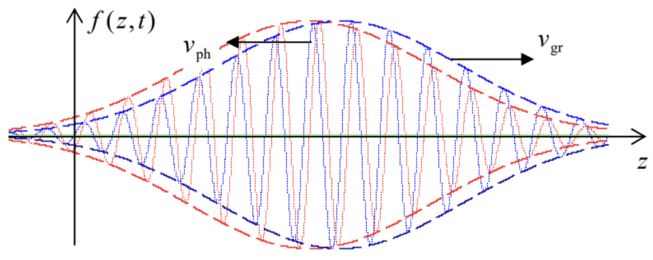
This fact may look strange, but is in no contradiction with any fundamental principle. Let me remind you that, according to the definition of the vector k, its direction shows the direction of the phase velocity νph=ω/k of a sinusoidal (and hence infinitely long) wave, which cannot be used, for example, for signaling. Such signaling (by sending wave packets – see Fig. 13) is possible only with the group velocity νgr=dω/dk. This velocity in left-hand materials is always positive (directed along the vector S).
Perhaps the most fascinating effect possible with left-hand materials is the wave refraction at their interfaces with the usual, right-handed materials – first predicted by V. Veselago in 1960. Consider the example shown in Fig. 14a. In the incident wave, arriving from a usual material, the directions of vectors k− and S− coincide, and so they are in the reflected wave with vectors k′− and S′−. This means that the electric and magnetic fields in the interface plane (z=0) are, at our choice of coordinates, proportional to exp{ikxx}, with a positive component kx=k−cosθ. To satisfy any linear boundary conditions, the refracted wave, propagating into the left-handed material, has to match that dependence, i.e. have a positive x-component of its wave vector k+. But in this medium, this vector has to be antiparallel to the vector S, which in turn should be directed out of the interface, because it represents the power flow from the interface into the material’s bulk. These conditions cannot be reconciled by the refracted wave propagating along the usual Snell-law direction (shown with the dashed line in Fig. 13a), but are all satisfied at refraction in the direction given by Snell’s angle with the opposite sign. (Hence the term “negative refraction”).39
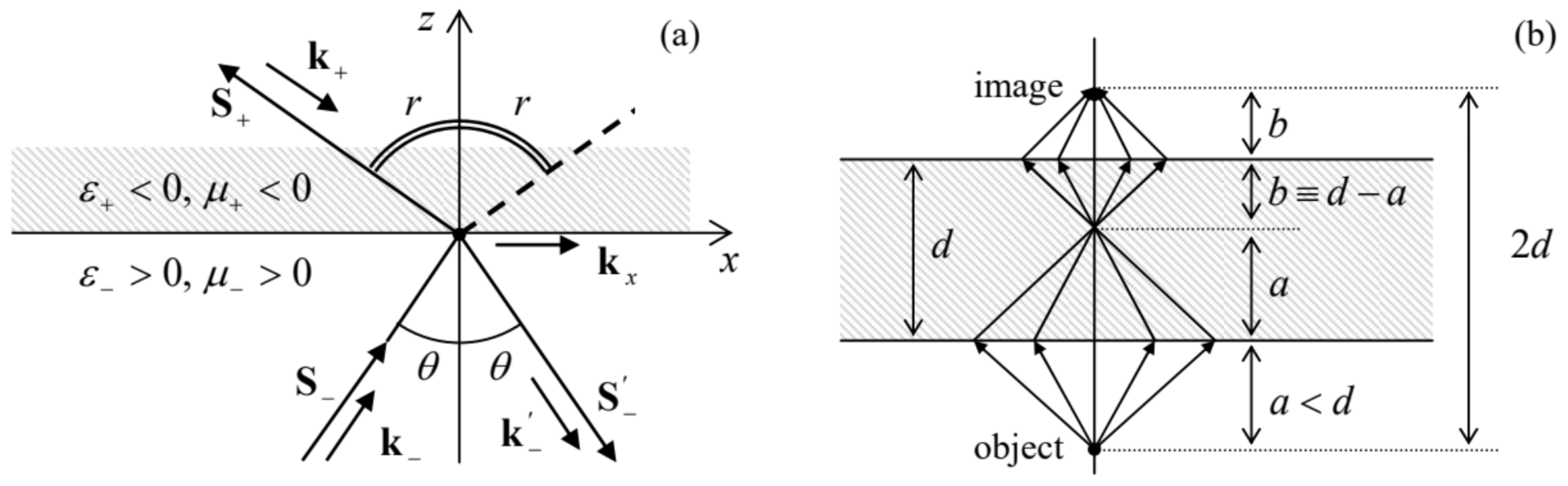
In order to understand how unusual the results of the negative refraction may be, let us consider a parallel slab of thickness d, made of a hypothetical left-handed material with exactly selected values ε=−ε0, and μ=−μ0 (see Fig. 14b). For such a material, placed in free space, the refraction angle r=−θ, so that the rays from a point source, located in free space, at a distance a<d from the slab, propagate as shown on that panel, i.e. all meet again at the distance a inside the plate, and then continue to propagate to the second surface of the slab. Repeating our discussion for this surface, we see that a point’s image is also formed beyond the slab, at distance 2a+2b=2a+2(d−a)=2d from the object.
Superficially, this system looks like a usual lens, but the well-known lens formula, which relates a and b with the focal length f, is not satisfied. (In particular, a parallel beam is not focused into a point at any finite distance.) As an additional difference from the usual lens, the system shown in Fig. 14b does not reflect any part of the incident light. Indeed, it is straightforward to check that for all the above formulas for R and T to be valid, the sign of the wave impedance Z in left-handed materials has to be kept positive. Thus, for our particular choice of parameters (ε=−ε0,μ=−μ0), Eqs. (91a) and (95a) are valid with Z+=Z−=Z0 and cosr=cosθ=1, giving R=0 for any linear polarization, and hence for any other wave polarization – circular, elliptic, natural, etc.
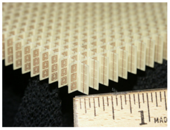
The perfect lens suggestion has triggered a wave of efforts to implement left-hand materials experimentally. (Attempts to find such materials in nature have failed so far.) Most progress in this direction has been achieved using the so-called metamaterials, which are essentially quasi-periodic arrays of specially designed electromagnetic resonators, ideally with high density n>>λ−3. For example, Fig. 15 shows the metamaterial that was used for the first demonstration of negative refractivity in the microwave region – for ~10-GHz frequencies.40 It combines straight strips of a metallic film, working as lumped resonators with a large electric dipole moment (hence strongly coupled to the wave’s electric field E), and several almost-closed film loops (so-called split rings), working as lumped resonators with large magnetic dipole moments, coupled to the field H. The negative refractivity is achieved by designing the resonance frequencies close to each other. More recently, metamaterials with negative refractivity were demonstrated in the optical range,41 although to the best of my knowledge, their relatively large absorption still prevents practical applications.
This progress has stimulated the development of other potential uses of metamaterials (not necessarily the left-handed ones), in particular, designs of nonuniform systems with engineered distributions ε(r,ω) and μ(r,ω) that may provide electromagnetic wave propagation along the desired paths, e.g., around a certain region of space, making it virtually invisible for an external observer – so far, within a limited frequency range.42
As was mentioned in Sec. 5.5, another way to reach negative values of μ(ω) is to place a ferromagnetic material into such an external dc magnetic field that the frequency ωr of the ferromagnetic resonance is somewhat lower than ω. If thin layers of such a material (e.g., nickel) are interleaved with
layers of a non-magnetic very good conductor (such as copper), the resulting metamaterial has an average value of μ(ω) – say, positive, but substantially below μ0. According to Eq. (6.33), the skin-depth δs of such a material may be larger than that of the good conductor alone, enforcing a more uniform distribution of the ac current flowing along the layers, and hence making the energy losses lower than in the good conductor alone. This effect may be useful, in particular, for electronic circuit interconnects.43
Reference
33 The latter relation is traditionally called the Snell law, after a 17th century astronomer Willebrord Snellius, but it has been traced all the way back to a circa 984 work by Abu Saad al-Ala ibn Sahl. (Claudius Ptolemy who performed pioneering experiments on light refraction in the 2nd century AD, was just one step from this result.)
34 Note that we may calculate the reflection and transmission coefficients R′ and T′ for the wave traveling in the opposite direction just by making the following parameter swaps: Z+↔Z− and θ↔r, and that the resulting coefficients satisfy the following Stokes relations: R′=−R, and R2+TT′=1, for any Z±.
35 Named after Augustin-Jean Fresnel (1788-1827), one of the wave optics pioneers, who is credited, among many other contributions (see, in particular, discussions in Ch. 8), for the concept of light as a purely transverse wave.
36 This effect is used in practice to obtain linearly polarized light, with the electric field vector perpendicular to the plane of incidence, from the natural light with its random polarization. An even more practical application of the effect is a partial reduction of undesirable glare from wet surfaces (for the water/air interface, n+/n−≈1.33, giving θB≈50∘) by making car headlight covers and glasses of vertically-polarizing materials.
37 A very simple interpretation of Eq. (96) is based on the fact that, together with the Snell law (82), it gives r+θ=π/2. As a result, the vector E+ is parallel to the vector k′−, and hence oscillating electric dipoles of the medium at z>0 do not have the component that could induce the transverse electric field E′− of the potential reflected wave.
38 Despite some important background theoretical work by A. Schuster (1904), L. Mandelstam (1945), D. Sivikhin (1957), and especially V. Veselago (1966-67), the negative refractivity effects became a subject of intensive scientific research and engineering development only in the 2000s. Note that these effects are not covered in typical E&M courses, so that the balance of this section may be skipped at first reading.
39 In some publications inspired by this fact, the left-hand materials are prescribed a negative index of refraction n. However, this prescription should be treated with care. For example, it complies with the first form of Eq. (84), but not its second form, and the sign of n, in contrast to that of the wave vector k, is a matter of convention.
40 R. Shelby et al., Science 292, 77 (2001); J. Wilson and Z. Schwartz, Appl. Phys. Lett. 86, 021113 (2005).
41 See, e.g., J. Valentine et al., Nature 455, 376 (2008).
42 For a review of such “invisibility cloaks”, see, e.g., B. Wood, Comptes Rendus Physique 10, 379 (2009).
43 See, for example, N. Sato et al., J. Appl. Phys. 111, 07A501 (2012), and references therein.