7.5: Transmission Lines- TEM Waves

So far, we have analyzed plane electromagnetic waves, implying that their cross-section is infinite – evidently, the unrealistic assumption. The cross-section may be limited, still sustaining wave propagation along wave transmission lines:⁴⁴ long, uniform structures made of either good conductors or dielectrics. Let us first discuss the first option, using the following simplifying assumptions:

(i) the structure is a cylinder (not necessarily with a round cross-section, see Fig. 16) filled with a usual (right-handed), uniform dielectric material with negligible energy losses \(\ \left(\varepsilon^{\prime \prime}=\mu^{\prime \prime}=0\right)\), and

(ii) the wave attenuation due to the skin effect is also negligibly low. (As Eq. (78) indicates, for that the characteristic size \(\ a\) of the line’s cross-section has to be much larger than the skin-depth \(\ \delta_{\mathrm{s}}\) of its wall material. The energy dissipation effects will be analyzed in Sec. 9 below.)

With such exclusion of energy losses, we may look for a particular solution of the macroscopic Maxwell equations in the form of a monochromatic wave traveling along the line:

\[\ \mathbf{E}(\mathbf{r}, t)=\operatorname{Re}\left[\mathbf{E}_{\omega}(x, y) e^{i\left(k_{z} z-\omega t\right)}\right], \quad \mathbf{H}(\mathbf{r}, t)=\operatorname{Re}\left[\mathbf{H}_{\omega}(x, y) e^{i\left(k_{z} z-\omega t\right)}\right],\tag{7.98}\]

with real \(\ k_{z}\), where the z-axis is directed along the transmission line – see Fig. 16. Note that this form allows an account for a substantial coordinate dependence of the electric and magnetic field within the plane \(\ [x, y]\) of the transmission line’s cross-section, as well as for longitudinal components of the fields, so that the solution (98) is substantially more complex than the plane waves we have discussed above. We will see in a minute that as a result of this dependence, the parameter \(\ k_{z}\) may be very much different from its plane-wave value (13), \(\ k \equiv \omega(\varepsilon \mu)^{1 / 2}\), in the same material, at the same frequency.

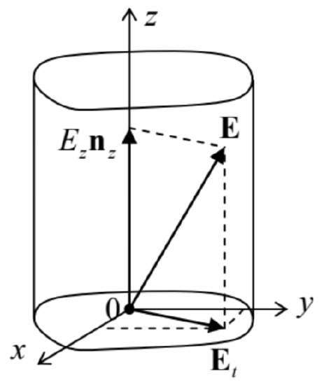Fig. 7.16. Electric field’s decomposition in a transmission line (in particular, a waveguide).

In order to describe these effects quantitatively, let us decompose the complex amplitudes of the wave’s fields into their longitudinal and transverse components (Fig. 16):⁴⁵

\[\ \mathbf{E}_{\omega}=E_{z} \mathbf{n}_{z}+\mathbf{E}_{t}, \quad \mathbf{H}_{\omega}=H_{z} \mathbf{n}_{z}+\mathbf{H}_{t}.\tag{7.99}\]

Plugging Eqs. (98)-(99) into the source-free Maxwell equations (2), and requiring the longitudinal and transverse components to be balanced separately, we get

\[\ \begin{array}{ll}
i k_{z} \mathbf{n}_{z} \times \mathbf{E}_{t}-i \omega \mu \mathbf{H}_{t}=-\nabla_{t} \times\left(E_{z} \mathbf{n}_{z}\right), & i k_{z} \mathbf{n}_{z} \times \mathbf{H}_{t}+i \omega \varepsilon \mathbf{E}_{t}=-\nabla_{t} \times\left(H_{z} \mathbf{n}_{z}\right), \\
\nabla_{t} \times \mathbf{E}_{t}=i \omega \mu H_{z} \mathbf{n}_{z}, & \nabla_{t} \times \mathbf{H}_{t}=-i \varepsilon \omega E_{z} \mathbf{n}_{z}, \\
\nabla_{t} \cdot \mathbf{E}_{t}=-i k_{z} E_{z}, & \nabla_{t} \cdot \mathbf{H}_{t}=-i k_{z} H_{z} .
\end{array}\tag{7.100}\]

where \(\ \nabla_{t}\) is the 2D del operator acting in the transverse plane \(\ [x, y]\) only, i.e. the usual \(\ \nabla\), but with \(\ \partial / \partial z=0\). The system of Eqs. (100) looks even bulkier than the original equations (2), but it is much simpler for analysis. Indeed, eliminating the transverse components from these equations (or, even simpler, just plugging Eq. (99) into Eqs. (3) and keeping only their z-components), we get a pair of self-consistent equations for the longitudinal components of the fields, ⁴⁶

\[\ \text{2D Helmholtz equations for } E_z \text{ and }H_z\quad\quad\quad\quad \left(\nabla_{t}^{2}+k_{t}^{2}\right) E_{z}=0, \quad\left(\nabla_{t}^{2}+k_{t}^{2}\right) H_{z}=0,\tag{7.101}\]

where \(\ k\) is still defined by Eq. (13), \(\ k=(\varepsilon \mu)^{1 / 2} \omega\), while

\[\ \text{Wave vector component balance}\quad\quad\quad\quad k_{t}^{2} \equiv k^{2}-k_{z}^{2}=\omega^{2} \varepsilon \mu-k_{z}^{2}\tag{7.102}\]

After the distributions \(\ E_{z}(x, y)\) and \(\ H_{z}(x, y)\) have been found from these equations, they provide right-hand sides for the rather simple, closed system of equations (100) for the transverse components of field vectors. Moreover, as we will see below, each of the following three types of solutions:

(i) with \(\ E_{z}=0\) and \(\ H_{z}=0\) (called the transverse electromagnetic, or \(\ TEM\) waves),

(ii) with \(\ E_{z}=0\), but \(\ H_{z} \neq 0\) (called either the \(\ TE\) waves or, more frequently, \(\ H\)-modes), and

(iii) with \(\ E_{z} \neq 0\), but \(\ H_{z}=0\) (the so-called \(\ TM\) waves or \(\ E\)-modes),

has its own dispersion law and hence its own wave propagation velocity; as a result, these modes (i.e. the field distribution patterns) may be considered separately.

In the balance of this section, we will focus on the simplest, TEM waves (i), with no longitudinal components of either field. For them, the top two equations of the system (100) immediately give Eqs. (6) and (13), and \(\ k_{z}=k\). In plain English, this means that \(\ \mathbf{E}=\mathbf{E}_{t}\) and \(\ \mathbf{H}=\mathbf{H}_{t}\) are proportional to each other and are mutually perpendicular (just as in the plane wave) at each point of the cross-section, and that the TEM wave’s impedance \(\ Z \equiv E / H\) and dispersion law \(\ \omega(k)\), and hence the propagation speed, are the same as in a plane wave in the same material. In particular, if \(\ \varepsilon\) and \(\ \mu\) are frequency-independent within a certain frequency range, the dispersion law within this range is linear, \(\ \omega=k /(\varepsilon \mu)^{1 / 2}\), and the wave’s speed does not depend on its frequency. For practical applications to telecommunications, this is a very important advantage of the TEM waves over their TM and TE counterparts – to be discussed below.

Unfortunately for practice, such waves cannot propagate in every transmission line. To show this, let us have a look at the two last lines of Eqs. (100). For the TEM waves \(\ \left(E_{z}=0, H_{z}=0, k_{z}=k\right)\), they are reduced to merely

\[\ \begin{array}{ll}
\nabla_{t} \times \mathbf{E}_{t}=0, & \nabla_{t} \times \mathbf{H}_{t}=0, \\
\nabla_{t} \cdot \mathbf{E}_{t}=0, & \nabla_{t} \cdot \mathbf{H}_{t}=0.
\end{array}\tag{7.103}\]

Within the coarse-grain description of the conducting walls of the line (i. e., neglecting the skin depth in comparison with the cross-section dimensions), we have to require that inside them, \(\ \mathbf{E}=\mathbf{H}=0\). Close to a wall but outside it, the normal component \(\ E_{n}\) of the electric field may be different from zero, because
surface charges may sustain its jump – see Sec. 2.1, in particular Eq. (2.3). Similarly, the tangential component \(\ H_{\tau}\) of the magnetic field may have a finite jump at the surface due to skin currents – see Sec. 6.3, in particular Eq. (6.38). However, the tangential component of the electric field and the normal component of the magnetic field cannot experience such jumps, and in order to have them equal to zero inside the walls they have to equal zero just outside the walls as well:

\[\ \mathbf{E}_{\tau}=0, \quad H_{n}=0.\tag{7.104}\]

But the left columns of Eqs. (103) and (104) coincide with the formulation of the 2D boundary problem of electrostatics for the electric field induced by electric charges of the conducting walls, with the only difference that in our current case the value of \(\ \varepsilon\) actually means \(\ \varepsilon(\omega)\). Similarly, the right columns of those relations coincide with the formulation of the 2D boundary problem of magnetostatics for the magnetic field induced by currents in the walls, with \(\ \mu \rightarrow \mu(\omega)\). The only difference is that in our current, coarse-grain approximation the magnetic fields cannot penetrate into the conductors.

Now we immediately see that in waveguides with a singly-connected wall, for example, a hollow conducting tube (see, e.g., Fig. 16), the TEM waves are impossible, because there is no way to create a non-zero electrostatic field inside a conductor with such cross-section. However, such fields (and hence the TEM waves) are possible in structures with cross-sections consisting of two or more disconnected (galvanically-insulated) parts – see, e.g., Fig. 17.

Fig. 7.17. An example of the cross-section of a transmission line that may support the TEM wave propagation.

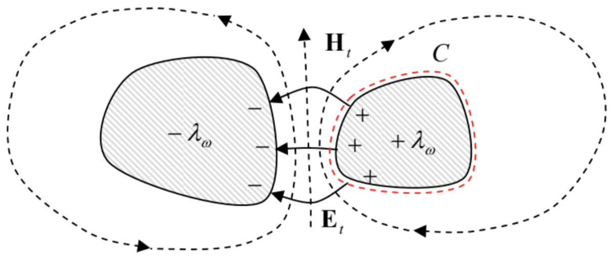
In order to derive “global” relations for such a transmission line, let us consider the contour \(\ C\) drawn very close to the surface of one of its conductors – see, e.g., the red dashed line in Fig. 17. We can consider it, on one hand, as the cross-section of a cylindrical Gaussian volume of a certain elementary length \(\ d z<<\lambda \equiv 2 \pi / k\). Using the generalized Gauss law (3.34), we get

\[\ \oint_{C}\left(\mathbf{E}_{t}\right)_{n} d r=\frac{\Lambda_{\omega}}{\varepsilon},\tag{7.105}\]

where \(\ \Lambda_{\omega}\) (not to be confused with the wavelength \(\ \lambda\)!) is the complex amplitude of the linear density of the electric charge of the conductor. On the other hand, the same contour \(\ C\) may be used in the generalized Ampère law (5.116) to write

\[\ \oint_{C}\left(\mathbf{H}_{t}\right)_{\tau} d r=I_{\omega},\tag{7.106}\]

where \(\ I_{\omega}\) is the total current flowing along the conductor (or rather its complex amplitude). But, as was mentioned above, in the TEM wave the ratio \(\ E_{t} / H_{t}\) of the field components participating in these two integrals is constant and equal to \(\ Z=(\mu / \varepsilon)^{1 / 2}\), so that Eqs. (105)-(106) give the following simple relation between the “global” variables of the conductor:

\[\ I_{\omega}=\frac{\Lambda_{\omega} / \varepsilon}{Z} \equiv \frac{\Lambda_{\omega}}{(\varepsilon \mu)^{1 / 2}} \equiv \frac{\omega}{k} \Lambda_{\omega}.\tag{7.107}\]

This important relation may be also obtained in a different way; let me describe it as well, because (as we will see below) it has an independent heuristic value. Let us consider a small segment \(\ dz<<\lambda=2 \pi / k\) of the line’s conductor, and apply the electric charge conservation law (4.1) to the instant values of the linear charge density and current. The cancellation of \(\ dz\) in both parts yields

\[\ \frac{\partial \Lambda(z, t)}{\partial t}=-\frac{\partial I(z, t)}{\partial z}.\tag{7.108}\]

If we accept the sinusoidal waveform, \(\ \exp \{i(k z-\omega t)\}\), for both these variables, we immediately recover Eq. (107) for their complex amplitudes, showing that this relation expresses just the charge continuity law.

The global equation (108) may be made more specific in the case when the frequency dependence of \(\ \varepsilon\) and \(\ \mu\) is negligible, and the transmission line consists of just two isolated conductors – see, e.g., Fig. 17. In this case, to have the wave localized in the space near the two conductors, we need a sufficiently fast decrease of its electric field at large distances. For that, their linear charge densities for each value of \(\ z\) should be equal and opposite, and we can simply relate them to the potential difference \(\ V\) between the conductors:

\[\ \frac{\Lambda(z, t)}{V(z, t)}=C_{0},\tag{7.109}\]

where \(\ C_{0}\) is the mutual capacitance of the conductors (per unit length) – which was repeatedly discussed in Chapter 2. Then Eq. (108) takes the following form:

\[\ C_{0} \frac{\partial V(z, t)}{\partial t}=-\frac{\partial I(z, t)}{\partial z}.\tag{7.110}\]

Next, let us consider the contour shown with the red dashed line in Fig. 18 (which shows a cross-section of the transmission line by a plane containing the wave propagation axis \(\ z\)), and apply to it the Faraday induction law (6.3).

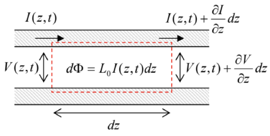Fig. 7.18. Electric current, magnetic flux, and voltage in a two-conductor transmission line.

Since, in the coarse-grain approximation, the electric field inside the conductors (in Fig. 18, on the horizontal segments of the contour) vanishes, the total e.m.f. equals the difference of the voltages \(\ V\) at the ends of the segment \(\ dz\), while the only source of the magnetic flux through the area limited by the contour is the (equal and opposite) currents \(\ \pm I\) in the conductors, we can use Eq. (5.70) to express it. As a result, canceling \(\ dz\) in both parts of the equation, we get

\[\ L_{0} \frac{\partial I(z, t)}{\partial t}=-\frac{\partial V(z, t)}{\partial z},\tag{7.111}\]

where \(\ L_{0}\) is the mutual inductance of the conductors per unit length. The only difference between this \(\ L_{0}\) and the dc mutual inductances discussed in Chapter 5 is that at the high frequencies we are analyzing now, \(\ L_{0}\) should be calculated neglecting the magnetic field penetration into the conductors. (In the dc case, we had the same situation for superconductor electrodes, within their coarse-grain, ideal-diamagnetic description.)

The system of Eqs. (110) and (111) is frequently called the telegrapher’s equations. Combined, they give for any “global” variable \(\ f\) (either \(\ V\), or \(\ I\), or \(\ \Lambda\)) the usual 1D wave equation,

\[\ \frac{\partial^{2} f}{\partial z^{2}}-L_{0} C_{0} \frac{\partial^{2} f}{\partial t^{2}}=0,\tag{7.112}\]

which describes dispersion-free TEM wave’s propagation. Again, this equation is only valid within the frequency range where the frequency dependence of both \(\ \varepsilon\) and \(\ \mu\) is negligible. If it is not so, the global approach may still be used for sinusoidal waves \(\ f=\operatorname{Re}\left[f_{\omega} \exp \{i(k z-\omega t)\}\right]\). Repeating the above arguments, instead of Eqs. (110)-(111) we get a more general system of two algebraic equations

\[\ \omega C_{0} V_{\omega}=k I_{\omega}, \quad \omega L_{0} I_{\omega}=k V_{\omega},\tag{7.113}\]

in which \(\ L_{0} \propto \mu\) and \(\ C_{0} \propto \varepsilon\) may now depend on frequency. These equations are consistent only if

\[\ L_{0} C_{0}=\frac{k^{2}}{\omega^{2}} \equiv \frac{1}{\nu^{2}} \equiv \varepsilon \mu. \quad\quad\quad\quad L_0C_0 \text{ product invariance}\tag{7.114}\]

Besides the fact we have already known (that the TEM wave’s speed is the same as that of the plane wave), Eq. (114) gives us the result that I confess was not emphasized enough in Chapter 5: the product \(\ L_{0} C_{0}\) does not depend on the shape or size of line’s cross-section provided that the magnetic field’s penetration into the conductors is negligible). Hence, if we have calculated the mutual capacitance \(\ C_{0}\) of a system of two cylindrical conductors, the result immediately gives us their mutual inductance: \(\ L_0=\varepsilon \mu / C_{0}\). This relationship stems from the fact that both the electric and magnetic fields may be expressed via the solution of the same 2D Laplace equation for the system’s cross-section.

With Eq. (114) satisfied, any of Eqs. (113) gives the same result for the following ratio:

\[\ Z_{W} \equiv \frac{V_{\omega}}{I_{\omega}}=\left(\frac{L_{0}}{C_{0}}\right)^{1 / 2},\quad\quad\quad\quad \text{Transmission line’s TEM Impedance}\tag{7.115}\]

which is called the transmission line’s impedance. This parameter has the same dimensionality (in SI units – ohms, denoted \(\ \Omega\)) as the wave impedance (7),

\[\ Z \equiv \frac{E_{\omega}}{H_{\omega}}=\left(\frac{\mu}{\varepsilon}\right)^{1 / 2},\tag{7.116}\]

but these parameters should not be confused, because \(\ Z_{W}\) depends on cross-section’s geometry, while \(\ Z\) does not. In particular, \(\ Z_{W}\) is the only important parameter of a transmission line for its matching with a lumped load circuit (Fig. 19) in the important case when both the cable cross-section’s size and the load’s linear dimensions are much smaller than the wavelength.⁴⁷

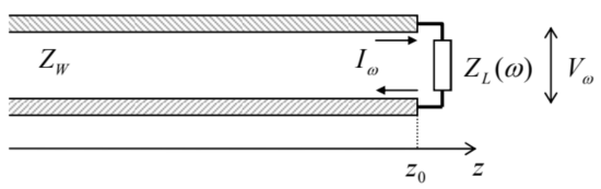Fig. 7.19. Passive, lumped termination of a TEM transmission line.

Indeed, in this case, we may consider the load in the quasistatic limit and write

\[\ V_{\omega}\left(z_{0}\right)=Z_{L}(\omega) I_{\omega}\left(z_{0}\right),\tag{7.117}\]

where \(\ Z_{L}(\omega)\) is the (generally complex) impedance of the load. Taking \(\ V(z, t)\) and \(\ I(z, t)\) in the form similar to Eqs. (61) and (62), and writing the two Kirchhoff’ s circuit laws for the point \(\ z=z_{0}\), we get for the reflection coefficient a result similar to Eq. (68):

\[\ R=\frac{Z_{L}(\omega)-Z_{W}}{Z_{L}(\omega)+Z_{W}}.\tag{7.118}\]

This formula shows that for the perfect matching (i.e. the total wave absorption in the load), the load’s impedance \(\ Z_{L}(\omega)\) should be real and equal to \(\ Z_{W}\) – but not necessarily to \(\ Z\).

As an example, let us consider one of the simplest (and most practically important) transmission lines: the coaxial cable (Fig. 20).⁴⁸

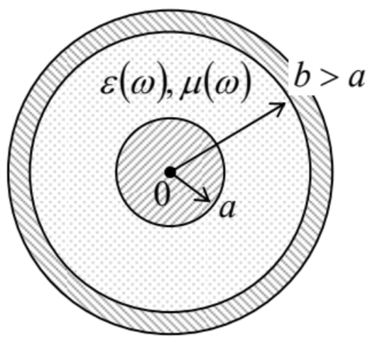Fig. 7. 20. The cross-section of a coaxial cable with (possibly, dispersive) dielectric filling.

For this geometry, we already know the expressions for both \(\ C_{0}\) and \(\ L_{0}\),⁴⁹ though they have to be modified for the dielectric and magnetic constants, and the magnetic field’s non-penetration into the conductors. As a result of such (elementary) modification, we get the formulas,

\[\ C_{0}=\frac{2 \pi \varepsilon}{\ln (b / a)}, \quad L_{0}=\frac{\mu}{2 \pi} \ln (b / a),\quad\quad\quad\quad \text{Coaxial cable’s }C_0 \text{ and }L_0\tag{7.119}\]

illustrating that the universal relationship (114) is indeed valid. For the cable’s impedance (115), Eqs. (119) yield a geometry-dependent value

\[\ Z_{W}=\left(\frac{\mu}{\varepsilon}\right)^{1 / 2} \frac{\ln (b / a)}{2 \pi} \equiv Z \frac{\ln (b / a)}{2 \pi} \neq Z.\tag{7.120}\]

For the standard TV antenna cables (such as RG-6/U, with \(\ b / a \sim 3, \varepsilon / \varepsilon_{0} \approx 2.2\)), \(\ Z_{W}=75 \Omega\), while for most computer component connections, coaxial cables with \(\ Z_{W}=50 \Omega\) (such as RG-58/U) are prescribed by electronic engineering standards. Such cables are broadly used for the transmission of electromagnetic waves with frequencies up to 1 GHz over distances of a few km, and up to ~20 GHz on the tabletop scale (a few meters), limited by wave attenuation – see Sec. 9 below.

Moreover, the following two facts enable a wide application, in electrical engineering and physical experiment, the coaxial-cable-like systems. First, as Eq. (5.78) shows, in a cable with \(\ a<<b\), most wave’s energy is localized near the internal conductor. Second, the theory to be discussed in the next section shows that excitation of other (\(\ H-\) and \(\ E-\)) waves in the cable are impossible until the wavelength \(\ \lambda\) becomes smaller than \(\ \sim \pi(a+b)\). As a result, the TEM mode propagation in a cable with \(\ a<<b<\lambda / \pi\) is not much affected even if the internal conductor is not straight, but is bent – for example, into a helix – see, e.g., Fig. 21.

Fig. 7.21. A typical traveling-wave tube: (1) electron gun, (2) ac input, (3) beam-focusing magnets, (4) wave attenuator, (5) helix coil, (6) ac output, (7) vacuum tube, (8) electron collector. Adapted from https://en.Wikipedia.org/wiki/Traveling-wave_tube under the Creative Commons BY-SA 3.0 license.

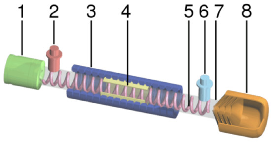
In such a system, called the traveling-wave tube, a quasi-TEM wave propagates, with velocity \(\ \nu=1 /(\varepsilon \mu)^{1 / 2} \sim c\), along the helix’ length, so that the velocity’s component along the cable’s axis may be made close to the velocity \(\ u<<c\) of the electron beam moving ballistically along the tube’s axis, enabling their effective interaction, and as a result, a length-accumulating amplification of the wave.⁵⁰

Another important example of a TEM transmission line is a set of two parallel wires. In the form of twisted pairs,⁵¹ they allow communications, in particular long-range telephone and DSL Internet connections, at frequencies up to a few hundred kHz, as well as relatively short, multi-line Ethernet and TV cables at frequencies up to ~ 1 GHz, limited mostly by the mutual interference (“crosstalk”) between the individual lines of the same cable, and the unintentional radiation of the wave into the environment.

---

Reference

⁴⁴ Another popular term is the waveguide, but it is typically reserved for the transmission lines with singly-connected cross-sections, to be analyzed in the next section. The first structure for guiding waves was proposed by J. J. Thomson in 1893, and experimentally tested by O. Lodge in 1894.

⁴⁵ For the notation simplicity, I am dropping index \(\ \omega\) in the complex amplitudes of the field components, and also have dropped the argument \(\ \omega\) in \(\ k_{z}\) and \(\ Z\), even though these parameters may depend on the wave’s frequency rather substantially – see below.

⁴⁶ The wave equation represented in the form (101), even with the 3D Laplace operator, is called the Helmholtz equation, named after Hermann von Helmholtz (1821-1894) – the mentor of H. Hertz and M. Planck, among many others.

⁴⁷ The ability of TEM lines to have such a small cross-section is their another important practical advantage.

⁴⁸ It was invented by the same O. Heaviside in 1880.

⁴⁹ See, respectively, Eqs. (2.49) and (5.79).

⁵⁰ Very unfortunately, in this course I will not have time/space to discuss even the (rather elegant) basic theory of such devices. The reader interested in this field may be referred, for example, to the detailed monograph by J. Whitaker, Power Vacuum Tubes Handbook, 3^rd ed., CRC Press, 2017.

⁵¹ Such twisting, around the line’s axis, reduces the crosstalk between adjacent lines, and the parasitic radiation at their bends.