8.9: Magnetic Dipole and Electric Quadrupole Radiation

Throughout this chapter, we have seen how many important results may be obtained from Eq. (26) for the electric dipole radiation by a small-size source (Fig. 1). Only in rare cases when this radiation is absent, for example, if the dipole moment p of the source equals zero (or does not change in time – either at all or at the frequency of our interest), higher-order effects may be important. I will discuss the main two of them, the quadrupole electric radiation and the dipole magnetic radiation.

In Sec. 2 above, the electric dipole radiation was calculated by plugging the expansion (19) into the exact formula (17b) for the retarded vector potential \(\ \mathbf{A}(\mathbf{r}, t)\). Let us make a more exact calculation, by keeping the second term of that expansion as well:

\[\ \mathbf{j}\left(\mathbf{r}^{\prime}, t-\frac{R}{\nu}\right) \approx \mathbf{j}\left(\mathbf{r}^{\prime}, t-\frac{r}{\nu}+\frac{\mathbf{r}^{\prime} \cdot \mathbf{n}}{\nu}\right) \equiv \mathbf{j}\left(\mathbf{r}^{\prime}, t^{\prime}+\frac{\mathbf{r}^{\prime} \cdot \mathbf{n}}{\nu}\right), \quad \text { where } t^{\prime} \equiv t-\frac{r}{\nu}.\tag{8.130}\]

Since the expansion is only valid if the last term in the time argument of \(\ \mathbf{j}\) is relatively small, in the Taylor expansion of \(\ \mathbf{j}\) with respect to that argument we may keep just two leading terms:

\[\ \mathbf{j}\left(\mathbf{r}^{\prime}, t^{\prime}+\frac{\mathbf{r}^{\prime} \cdot \mathbf{n}}{\nu}\right) \approx \mathbf{j}\left(\mathbf{r}^{\prime}, t^{\prime}\right)+\frac{\partial \mathbf{j}\left(\mathbf{r}^{\prime}, t^{\prime}\right)}{\partial t^{\prime}} \frac{\left(\mathbf{r}^{\prime} \cdot \mathbf{n}\right)}{\nu},\tag{8.131}\]

so that Eq. (17b) yields \(\ \mathbf{A}=\mathbf{A}_{d}+\mathbf{A}^{\prime}\), where \(\ \mathbf{A}_{\mathrm{d}}\) is the electric dipole contribution as given by Eq. (23), and \(\ \mathbf{A} \text {' }\) is the new term of the next order in the small parameter \(\ r^{\prime}<<r\):

\[\ \mathbf{A}^{\prime}(\mathbf{r}, t)=\frac{\mu}{4 \pi r \nu} \frac{\partial}{\partial t^{\prime}} \int \mathbf{j}\left(\mathbf{r}^{\prime}, t^{\prime}\right)\left(\mathbf{r}^{\prime} \cdot \mathbf{n}\right) d^{3} r^{\prime}.\tag{8.132}\]

Just as it was done in Sec. 2, let us evaluate this term for a system of non-relativistic particles with electric charges \(\ q_{k}\) and radius-vectors \(\ \mathbf{r}_{k}(t)\):

\[\ \mathbf{A}^{\prime}(\mathbf{r}, t)=\frac{\mu}{4 \pi r \nu}\left[\frac{d}{d t} \sum_{k} q_{k} \dot{\mathbf{r}}_{k}\left(\mathbf{r}_{k} \cdot \mathbf{n}\right)\right]_{t=t^{\prime}}.\tag{8.133}\]

Using the “bac minus cab” identity of the vector algebra again,⁴⁸ the vector operand of Eq. (133) may be rewritten as

\[\ \begin{aligned}
\dot{\mathbf{r}}_{k}\left(\mathbf{r}_{k} \cdot \mathbf{n}\right) & \equiv \frac{1}{2} \dot{\mathbf{r}}_{k}\left(\mathbf{r}_{k} \cdot \mathbf{n}\right)+\frac{1}{2} \dot{\mathbf{r}}_{k}\left(\mathbf{n} \cdot \mathbf{r}_{k}\right)=\frac{1}{2}\left(\mathbf{r}_{k} \times \dot{\mathbf{r}}_{k}\right) \times \mathbf{n}+\frac{1}{2} \mathbf{r}_{k}\left(\mathbf{n} \cdot \dot{\mathbf{r}}_{k}\right)+\frac{1}{2} \dot{\mathbf{r}}_{k}\left(\mathbf{n} \cdot \mathbf{r}_{k}\right) \\
& \equiv \frac{1}{2}\left(\mathbf{r}_{k} \times \dot{\mathbf{r}}_{k}\right) \times \mathbf{n}+\frac{1}{2} \frac{d}{d t}\left[\mathbf{r}_{k}\left(\mathbf{n} \cdot \mathbf{r}_{k}\right)\right],
\end{aligned}\tag{8.134}\]

so that the right-hand side of Eq. (133) may be represented as a sum of two terms, \(\ \mathbf{A}^{\prime}=\mathbf{A}_{\mathrm{m}}+\mathbf{A}_{\mathrm{q}}\), where

\[\ \mathbf{A}_{\mathrm{m}}(\mathbf{r}, t)=\frac{\mu}{4 \pi r \nu} \dot{\mathbf{m}}\left(t^{\prime}\right) \times \mathbf{n} \equiv \frac{\mu}{4 \pi r \nu} \dot{\mathbf{m}}\left(t-\frac{r}{\nu}\right) \times \mathbf{n}, \quad \text { with } \mathbf{m}(t) \equiv \frac{1}{2} \sum_{k} \mathbf{r}_{k}(t) \times q_{k} \dot{\mathbf{r}}_{k}(t);\tag{8.135}\]

\[\ \mathbf{A}_{\mathrm{q}}(\mathbf{r}, t)=\frac{\mu}{8 \pi r \nu}\left[\frac{d^{2}}{d t^{2}} \sum_{k} q_{k} \mathbf{r}_{k}\left(\mathbf{n} \cdot \mathbf{r}_{k}\right)\right]_{t=t^{\prime}}.\tag{8.136}\]

Comparing the second of Eqs. (135) with Eq. (5.91), we see that m is just the total magnetic moment of the source. On the other hand, the first of Eqs. (135) is absolutely similar in structure to Eq. (23), with p replaced with \(\ (\mathbf{m} \times \mathbf{n}) / \nu\), so that for the corresponding component of the magnetic field it gives (in the same approximation \(\ r >> \lambda\)) a result similar to Eq. (24):

\[\ \text{Magnetic dipole radiation: field}\quad\quad\quad\quad \mathbf{B}_{\mathrm{m}}(\mathbf{r}, t)=\frac{\mu}{4 \pi r \nu} \nabla \times\left[\dot{\mathbf{m}}\left(t-\frac{r}{\nu}\right) \times \mathbf{n}\right]=-\frac{\mu}{4 \pi r \nu^{2}} \mathbf{n} \times\left[\ddot{\mathbf{m}}\left(t-\frac{r}{\nu}\right) \times \mathbf{n}\right].\tag{8.137}\]

According to this expression, just as at the electric dipole radiation, the vector B is perpendicular to the vector n, and its magnitude is also proportional to \(\ \sin \Theta\), where \(\ \Theta\) is now the angle between the direction toward the observation point and the second time derivative of the vector m – rather than p:

\[\ B_{\mathrm{m}}=\frac{\mu}{4 \pi r \nu^{2}} \ddot{m}\left(t-\frac{r}{\nu}\right) \sin \Theta.\tag{8.138}\]

As the result, the intensity of this magnetic dipole radiation has a similar angular distribution:

\[\ \text{Magnetic dipole radiation: power}\quad\quad\quad\quad S_{r}=Z H^{2}=\frac{Z}{\left(4 \pi \nu^{2} r\right)^{2}}\left[\ddot{m}\left(t-\frac{r}{\nu}\right)\right]^{2} \sin ^{2} \Theta\tag{8.139}\]

- cf. Eq. (26), besides the (generally) different meaning of the angle \(\ \Theta\).

Note, however, that this radiation is usually much weaker than its electric-dipole counterpart. For example, for a non-relativistic particle with electric charge \(\ q\), moving on a trajectory of linear size \(\ \sim a\), the electric dipole moment is of the order of \(\ qa\), while its magnetic moment scales as \(\ q a^{2} \omega\), where \(\ \omega\) is the motion frequency. As a result, the ratio of the magnetic and electric dipole radiation intensities is of the order of \(\ (a \omega / \nu)^{2}\), i.e. the squared ratio of the particle’s speed to the speed of emitted waves – that has to be much smaller than 1 for our non-relativistic calculation to be valid.

The angular distribution of the electric quadrupole radiation, described by Eq. (136), is more complicated. To show this, we may add to \(\ \mathbf{A}_{\mathrm{q}}\) a vector parallel to n (i.e. along the wave’s propagation), getting

\[\ \mathbf{A}_{\mathrm{q}}(\mathbf{r}, t) \rightarrow \frac{\mu}{24 \pi r \nu} \ddot{\mathscr{Q}}\left(t-\frac{r}{\nu}\right), \quad \text { where } \mathscr{Q} \equiv \sum_{k} q_{k}\left\{3 \mathbf{r}_{k}\left(\mathbf{n} \cdot \mathbf{r}_{k}\right)-\mathbf{n} r_{k}^{2}\right\},\tag{8.140}\]

because this addition does not give any contribution to the transverse component of the electric and magnetic fields, i.e. to the radiated wave. According to the above definition of the vector \(\ \mathscr{Q}\), its Cartesian components may be represented as

\[\ \mathscr{Q}_{j}=\sum_{j^{\prime}=1}^{3} \mathscr{Q}_{j j^{\prime}} n_{j^{\prime}},\tag{8.141}\]

where \(\ \mathscr{Q}_{j j’}\) are the elements of the electric quadrupole tensor of the system – see the last of Eqs. (3.4):

\[\ \mathscr{Q}_{j j^{\prime}}=\sum_{k} q_{k}\left(3 r_{j} r_{j^{\prime}}-r^{2} \delta_{j j^{\prime}}\right)_{k}.\tag{8.142}\]

(Let me hope that the reader has already acquired some experience in the calculation of this tensor’s components – e.g., for the simple systems specified in Problems 3.2 and 3.3.) Now taking the curl of the first of Eqs. (140) at \(\ r >> \lambda\), we get

\[\ \mathbf{B}_{\mathrm{q}}(\mathbf{r}, t)=-\frac{\mu}{24 \pi r \nu^{2}} \mathbf{n} \times \dddot{\mathscr{Q}}\left(t-\frac{r}{\nu}\right).\quad\quad\quad\quad\text{Electric quadrupole radiation: field}\tag{8.143}\]

This expression is similar to Eqs. (24) and (137), but according to Eqs. (140) and (142), components of the vector \(\ \mathscr{Q}\) do depend on the direction of the vector n, leading to a different angular dependence of \(\ S_{r}\).

As the simplest example, let us consider the system of two equal point electric charges moving symmetrically, at equal distances \(\ d(t)<<\lambda\) from a stationary center – see Fig. 16.

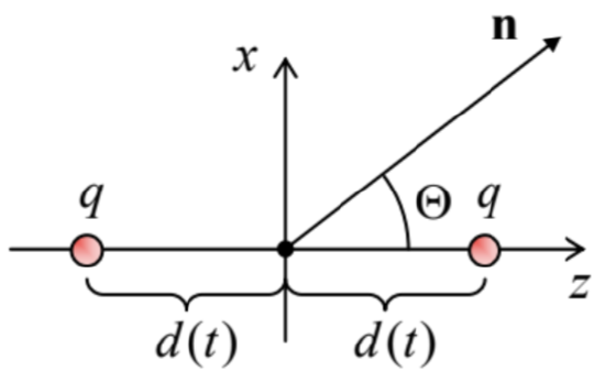Fig. 8.16. The simplest system emitting electric quadrupole radiation.

Due to the symmetry of the system, its dipole moments p and m (and hence its electric and magnetic dipole radiation) vanish, but the quadrupole tensor (142) still has non zero components. With the coordinate choice shown in Fig. 16, these components are diagonal:

\[\ \mathscr{Q}_{x x}=\mathscr{Q}_{y y}=-2 q d^{2}, \quad \mathscr{Q}_{z z}=4 q d^{2}.\tag{8.144}\]

With the x-axis selected within the common plane of the z-axis and the direction n toward the source (Fig. 16), so that \(\ n_{x}=\sin \Theta\), \(\ n_{y}=0\), and \(\ n_{z}=\cos \Theta\), Eq. (141) yields

\[\ \mathscr{Q}_{x}=-2 q d^{2} \sin \Theta, \quad \mathscr{Q}_{y}=0, \quad \mathscr{Q}_{z}=4 q d^{2} \cos \Theta,\tag{8.145}\]

and the vector product in Eq. (143) has only one non-vanishing Cartesian component:

\[\ (\mathbf{n} \times \dddot{\mathscr{Q}})_{y}=n_{z} \dddot{\mathscr{Q}}_{x}-n_{x} \ddot{\mathscr{Q}}_{z}=-6 q \sin \Theta \cos \Theta \frac{d^{3}}{d t^{3}}\left[d^{2}(t)\right].\tag{8.146}\]

As a result, the quadrupole radiation intensity, \(\ S \propto B_{\mathrm{q}}^{2}\), is proportional to \(\ \sin ^{2} \Theta \cos ^{2} \Theta\), i.e. vanishes not only along the symmetry axis of the system (as the electric-dipole and the magnetic-dipole radiations would do), but also in all directions perpendicular to this axis, reaching its maxima at \(\ \Theta=\pm \pi / 4\).

For more complex systems, the angular distribution of the electric quadrupole radiation may be different, but it may be proved that its total (instant) power always obeys the following simple formula:

\[\ \text{Electric quadrupole radiation: power}\quad\quad\quad\quad \mathscr{P}_{q}=\frac{Z}{1440 \pi \nu^{4}} \sum_{j, j^{\prime}=1}^{3}\left(\mathscr{\dddot{Q}}_{j j^{\prime}}\right)^{2}.\tag{8.147}\]

Let me finish this section by giving, also without proof, one more fact important for some applications: due to their different spatial structure, the magnetic-dipole and electric quadrupole radiation fields do not interfere, i.e. the total power of radiation (neglecting the electric-dipole and higher multipole terms) may be found as the sum of these components, calculated independently. On the contrary, if the electric-dipole and magnetic-dipole radiations of the same system are comparable, they typically interfere coherently, so that their radiation fields (rather than powers) should be summed up.

---

Reference

⁴⁸ If you still need it, see MA Eq. (7.5).