8.10: Exercise Problems

8.1. In the electric-dipole approximation, calculate the angular distribution and the total power of electromagnetic radiation by the hydrogen atom within the following classical model: an electron rotating, at a constant distance \(\ R\), about a much heavier proton. Use the latter result to evaluate the classical lifetime of the atom, borrowing the initial value of \(\ R\) from quantum mechanics: \(\ R(0)=r_{\mathrm{B}} \approx 0.53\times10^{-10}\mathrm{m}\).

8.2. A non-relativistic particle of mass \(\ m\), with electric charge \(\ q\), is placed into a uniform magnetic field B. Derive the law of decrease of the particle’s kinetic energy due to its electromagnetic radiation at the cyclotron frequency \(\ \omega_{\mathrm{c}}=q B / m\). Evaluate the rate of such radiation cooling of electrons in a magnetic field of 1 T, and estimate the energy interval in which this result is quantitatively correct.

Hint: The cyclotron motion will be discussed in detail (for arbitrary particle velocities \(\ \nu \sim c\)) in Sec. 9.6 below, but I hope that the reader knows that in the non-relativistic case (\(\ \nu<<c\)) the above formula for \(\ \omega_{\mathrm{c}}\) may be readily obtained by combining the 2^nd Newton law \(\ m \nu_{\perp}^{2} / R=q \nu_{\perp} B\) for the circular motion of the particle under the effect of the magnetic component of the Lorentz force (5.10), and the geometric relation \(\ \nu_{\perp}=R \omega_{\mathrm{c}}\). (Here \(\ \mathbf{v}_{\perp}\) is particle’s velocity in the plane normal to the vector B.)

8.3. Solve the dipole antenna radiation problem discussed in Sec. 2 (see Fig. 3) for the optimal length \(\ l=\lambda / 2\), assuming that the current distribution in each of its arms is sinusoidal: \(\ I(z, t)=I_{0} \cos (\pi z / l)\cos\omega t\).⁴⁹

8.4. Use the Lorentz oscillator model of a bound charge, given by Eq. (7.30), to explore the transition between the two scattering limits discussed in Sec. 3, and in particular, the resonant scattering taking place at \(\ \omega \approx \omega_{0}\). In this context, discuss the contribution of scattering into the oscillator’s damping.

8.5.^* A sphere of radius \(\ R\), made of a material with a uniform permanent electric polarization \(\ \mathbf{P}_{0}\) and a constant mass density \(\ \rho\), is free to rotate about its center. Calculate the average total cross-section of scattering, by the sphere, of a linearly polarized electromagnetic wave of frequency \(\ \omega<<R / c\), propagating in free space, in the limit of small wave amplitude, assuming that the initial orientation of the polarization vector \(\ \mathbf{P}_{0}\) is random.

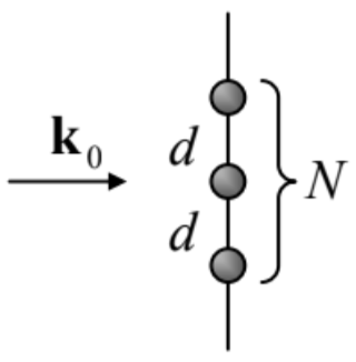
8.6. Use Eq. (56) to analyze the interference/diffraction pattern produced by a plane wave’s scattering on a set of \(\ N\) similar, equidistant points on a straight line normal to the direction of the incident wave’s propagation – see the figure on the right. Discuss the trend(s) of the pattern in the limit \(\ N \rightarrow \infty\).

8.7. Use the Born approximation to calculate the differential cross-section of the plane wave scattering by a uniform dielectric sphere of an arbitrary radius \(\ R\). In the limits \(\ k R<<1\) and \(\ 1<<k R\) (where \(\ k\) is the wave number), analyze the angular dependence of the differential cross-section and calculate the total cross-section of scattering.

8.8. A sphere of radius \(\ R\) is made of a uniform dielectric material, with an arbitrary dielectric constant. Derive an exact expression for its total cross-section of scattering of a low-frequency monochromatic wave, with \(\ k<<1 / R\), and compare the result with the solution of the previous problem.

8.9. Use the Born approximation to calculate the differential cross-section of the plane wave scattering on a right, circular cylinder of length \(\ l\) and radius \(\ R\), for an arbitrary angle of incidence.

8.10. Formulate the quantitative condition of the Born approximation’s validity for a uniform dielectric scatterer, with all linear dimensions of the order of the same scale \(\ a\).

8.11. If a scatterer absorbs some part of the incident wave’s power, it may be characterized by an absorption cross-section \(\ \sigma_{\mathrm{a}}\) defined similarly to Eq. (39) for the scattering cross-section:

\(\ \sigma_{\mathrm{a}} \equiv \frac{\overline{\mathscr{P}}_{a}}{\left|E_{\omega}\right|^{2} / 2 Z_{0}},\)

where the numerator is the time-averaged power absorbed is the scatterer. Calculate \(\ \sigma_{\mathrm{a}}\) for a very small sphere of radius \(\ R<<k^{-1}\), \(\ \delta_{\mathrm{s}}\), made of a nonmagnetic material with Ohmic conductivity \(\ \sigma\), and with high-frequency permittivity \(\ \varepsilon_{\mathrm{opt}}=\varepsilon_{0}\). Can \(\ \sigma_{\mathrm{a}}\) of such a sphere be larger than its geometric cross-section \(\ \pi R^{2}\)?

8.12. Use the Huygens principle to calculate wave’s intensity on the symmetry plane of the slit diffraction experiment (i.e. at \(\ x=0\) in Fig. 12), for arbitrary ratio \(\ z / k a^{2}\).

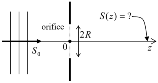
8.13. A plane wave with wavelength \(\ \lambda\) is normally incident on an opaque, plane screen, with a round orifice of radius \(\ R >> \lambda\). Use the Huygens principle to calculate the passing wave’s intensity distribution along the system’s symmetry axis, at distances \(\ z >> R\) from the screen (see the figure on the right), and analyze the result.

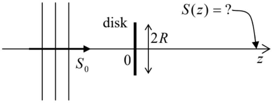
8.14. A plane monochromatic wave is now normally incident on an opaque circular disk of radius \(\ R>> \lambda\). Use the Huygens principle to calculate the wave’s intensity at distance \(\ z >> R\) behind the disk’s center (see the figure on the right). Discuss the result.

8.15. Use the Huygens principle to analyze the Fraunhofer diffraction of a plane wave normally incident on a square-shaped hole, of size \(\ a \times a\), in an opaque screen. Sketch the diffraction pattern you would observe at a sufficiently large distance, and quantify expression “sufficiently large” for this case.

8.16. Use the Huygens principle to analyze the propagation of a monochromatic Gaussian beam, described by Eq. (7.181), with the initial characteristic width \(\ a_{0} >> \lambda\), in a uniform, isotropic medium. Use the result for a semi-quantitative derivation of the so-called Abbe limit⁵⁰ for the spatial resolution of an optical system: \(\ w_{\min }=\lambda / 2 \sin \theta\), where \(\ \theta\) is the half-angle of the wave cone propagating from the object, and captured by the system.

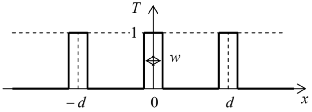
8.17. Within the Fraunhofer approximation, analyze the pattern produced by a 1D diffraction grating with the periodic transparency profile shown in the figure on the right, for the normal incidence of a plane, monochromatic wave.

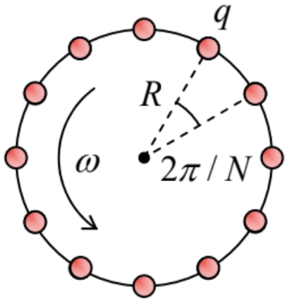
8.18. \(\ N\) equal point charges are attached, at equal intervals, to a circle rotating with a constant angular velocity about its center – see the figure on the right. For what values of \(\ N\) does the system emit:

(i) the electric dipole radiation?

(ii) the magnetic dipole radiation?

(iii) the electric quadrupole radiation?

8.19. What general statements can you make about:

(i) the electric dipole radiation, and

(ii) the magnetic dipole radiation,

due to a collision of an arbitrary number of similar classical, non-relativistic particles?

8.20. Calculate the angular distribution and the total power radiated by a small round loop antenna with radius \(\ R\), fed with ac current \(\ I(t)\) with frequency \(\ \omega\) and amplitude \(\ I_{0}\), into the free space.

8.21. The orientation of a magnetic dipole m, of a fixed magnitude, is rotating about a certain axis with angular velocity \(\ \omega\), with angle \(\ \alpha\) between them staying constant. Calculate the angular distribution and the average power of its radiation (into the free space).

8.22. Solve Problem 8 (also in the low-frequency limit \(\ k R<<1\)), for the case when the sphere’s material has a frequency-independent Ohmic conductivity \(\ \sigma\), and \(\ \varepsilon_{\mathrm{opt}}=\varepsilon_{0}\), in two limits:

(i) of a very large skin depth \(\ \left(\delta_{\mathrm{s}} >>R\right)\), and

(ii) of a very small skin depth \(\ \left(\delta_{\mathrm{s}}<<R\right)\).

8.23. Complete the solution of the problem started in Sec. 9, by calculating the full power of radiation of the system of two charges oscillating in antiphase along the same straight line – see Fig. 16. Also, calculate the average radiation power for the case of harmonic oscillations, \(\ d(t)=a \cos \omega t\), compare it with the case of a single charge performing similar oscillations, and interpret the difference.

---

Reference

⁴⁹ As was emphasized in Sec. 2, this is a reasonable guess rather than a controllable approximation. The exact (rather involved!) theory shows that this assumption gives errors ~5%, depending on the arm wire’s diameter.

⁵⁰ Reportedly, due to not only Ernst Abbe (1873), but also to Hermann von Helmholtz (1874).