8.8: Fraunhofer Diffraction from More Complex Scatterers

So far, our quantitative analysis of diffraction has been limited to a very simple geometry – a single slit in an otherwise opaque screen (Fig. 12). However, in the most important Fraunhofer limit, \(\ z>> k a^{2}\), it is easy to get a very simple expression for the plane wave diffraction/interference by a plane orifice (with a linear size \(\ \sim a\)) of arbitrary shape. Indeed, the evident 2D generalization of the approximation (106)-(107) is

\[\ \begin{aligned}
I_{x} I_{y} &=\int_{\text {orifice }} \exp \frac{i k\left[\left(x-x^{\prime}\right)^{2}+\left(y-y^{\prime}\right)^{2}\right]}{2 z} d x^{\prime} d y^{\prime} \\
& \approx \exp \left\{\frac{i k\left(x^{2}+y^{2}\right)}{2 z}\right\} \int_{\text {orifice }} \exp \left\{-i \frac{k x x^{\prime}}{z}-i \frac{k y y^{\prime}}{z}\right\} d x^{\prime} d y^{\prime}
\end{aligned}\tag{8.115}\]

so that besides the inconsequential total phase factor, Eq. (105) is reduced to

\[\ \text{General Fraunhofer diffraction pattern}\quad\quad\quad\quad f(\boldsymbol{\rho}) \propto f_{0} \int_{\text {orifice }} \exp \left\{-i \boldsymbol{\kappa} \cdot \boldsymbol{\rho}^{\prime}\right\} d^{2} \rho^{\prime} \equiv f_{0} \int_{\text {all screen }} T\left(\boldsymbol{\rho}^{\prime}\right) \exp \left\{-i \boldsymbol{\kappa} \cdot \boldsymbol{\rho}^{\prime}\right\} d^{2} \rho^{\prime}.\tag{8.116}\]

Here the 2D vector \(\ \boldsymbol{\kappa}\) (not to be confused with wave vector k, which is virtually perpendicular to \(\ \boldsymbol{\kappa!}\)) is defined as

\[\ \boldsymbol{\kappa} \equiv k \frac{\boldsymbol{\rho}}{z} \approx \mathbf{q} \equiv \mathbf{k}-\mathbf{k}_{0},\tag{8.117}\]

and \(\ \boldsymbol{\rho}=\{x, y\}\) and \(\ \boldsymbol{\rho^{\prime}}=\left\{x^{\prime}, y^{\prime}\right\}\) are 2D radius-vectors in the, respectively, observation and orifice planes – both nearly normal to the vectors \(\ \mathbf{k}\) and \(\ \mathbf{k}_{0}\). In the last form of Eq. (116), the function \(\ T\left(\rho^{\prime}\right)\) describes the screen’s transparency at point \(\ \boldsymbol{\rho’}\), and the integral is over the whole screen plane \(\ z^{\prime}=0\). (Though the two forms of Eq. (116) are strictly equivalent only if \(\ T\left(\rho^{\prime}\right)\) is equal to either 1 or 0, its last form may be readily obtained from Eq. (91) with \(\ f\left(r^{\prime}\right)=T\left(\rho^{\prime}\right) f_{0}\) for any transparency profile, provided that \(\ T\left(\rho^{\prime}\right)\) is any function that changes substantially only at distances much larger than \(\ \lambda \equiv 2 \pi / k\).)

From the mathematical point of view, the last form of Eq. (116) is just the 2D spatial Fourier transform of the function \(\ T\left(\rho^{\prime}\right)\), with the variable \(\ \boldsymbol{\kappa}\) defined by the observation point’s position: \(\ \boldsymbol{\rho}\equiv(z / k) \boldsymbol{\kappa} \equiv(z \lambda / 2 \pi) \boldsymbol{\kappa}\). This interpretation is useful because of the experience we all have with the Fourier transform, if only in the context of its time/frequency applications. For example, if the orifice is a single small hole, \(\ T\left(\rho^{\prime}\right)\) may be approximated by a delta function, so that Eq. (116) yields \(\ |f(\rho)| \approx \text { const }\). This result corresponds (at least for the small diffraction angles \(\ \theta \equiv \rho / z\), for which the Huygens approximation is valid) to a spherical wave spreading from the point-like orifice. Next, for two small holes, Eq. (116) immediately gives the interference pattern (103). Let me now use Eq. (116) to analyze other simplest (and most important) 1D transparency profiles, leaving 2D cases for the reader’s exercise.

(i) A single slit of width a (Fig. 12) may be described by transparency

\[\ T\left(\boldsymbol{\rho}^{\prime}\right)= \begin{cases}1, & \text { for }\left|x^{\prime}\right|<a / 2, \\ 0, & \text { otherwise}.\end{cases}\tag{8.118}\]

Its substitution into Eq. (116) yields

\[\ f(\boldsymbol{\rho}) \propto f_{0} \int_{-a / 2}^{+a / 2} \exp \left\{-i \kappa_{x} x^{\prime}\right\} d x^{\prime}=f_{0} \frac{\exp \left\{-i \kappa_{x} a / 2\right\}-\exp \left\{i \kappa_{x} a / 2\right\}}{-i \kappa_{x}} \propto \operatorname{sinc}\left(\frac{\kappa_{x} a}{2}\right)=\operatorname{sinc}\left(\frac{k x a}{2 z}\right),\tag{8.119}\]

naturally returning us to Eqs. (64) and (110), and hence to the red lines in Fig. 8 for the wave intensity. (Please note again that Eq. (116) describes only the Fraunhofer, but not the Fresnel diffraction!)

(ii) Two infinitely narrow, similar, parallel slits with a larger distance \(\ a\) between them (i.e. the simplest model of Young’s two-slit experiment) may be described by taking

\[\ T\left(\boldsymbol{\rho}^{\prime}\right) \propto \delta\left(x^{\prime}-a / 2\right)+\delta\left(x^{\prime}+a / 2\right),\tag{8.120}\]

so that Eq. (116) yields the generic 1D interference pattern,

\[\ f(\boldsymbol{\rho}) \propto f_{0}\left[\exp \left\{-\frac{i \kappa_{x} a}{2}\right\}+\exp \left\{\frac{i \kappa_{x} a}{2}\right\}\right] \propto \cos \frac{\kappa_{x} a}{2}=\cos \frac{k x a}{2 z},\tag{8.121}\]

whose intensity is shown with the blue line in Fig. 8.

(iii) In a more realistic model of Young’s experiment, each slit has a width (say, \(\ w\)) that is much larger than the light wavelength \(\ \lambda\), but still much smaller than the slit spacing \(\ a\). This situation may be described by the following transparency function

\[\ T\left(\boldsymbol{\rho}^{\prime}\right)=\sum_{\pm} \begin{cases}1, & \text { for }\left|x^{\prime} \pm a / 2\right|<w / 2, \\ 0, & \text { otherwise },\end{cases}\tag{8.122}\]

for which Eq. (116) yields a natural combination of the results (119) (with \(\ a\) replaced with w) and (121):

\[\ f(\mathbf{r}) \propto \operatorname{sinc}\left(\frac{k x w}{2 z}\right) \cos \left(\frac{k x a}{2 z}\right).\tag{8.123}\]

This is the usual interference pattern, but modulated with a Fraunhofer-diffraction envelope – shown in Fig. 15 with the dashed blue line. Since the function \(\ \operatorname{sinc}^{2} \xi\) decreases very fast beyond its first zeros at \(\ \xi=\pm \pi\), the practical number of observable interference fringes is close to \(\ 2a/w\).

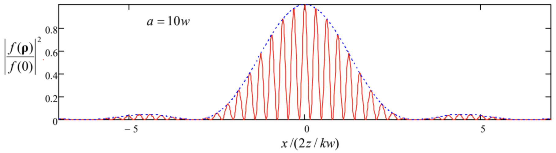Fig. 8.15. Young’s double-slit interference pattern for a finite-width slit.

(iv) A structure very useful for experimental and engineering practice is a set of many parallel, similar slits, called the diffraction grating.⁴⁶ If the slit width is much smaller than period \(\ d\) of the grating, its transparency function may be approximated as

\[\ T\left(\boldsymbol{\rho}^{\prime}\right) \propto \sum_{n=-\infty}^{+\infty} \delta\left(x^{\prime}-n d\right),\tag{8.124}\]

and Eq. (116) yields

\[\ f(\boldsymbol{\rho}) \propto \sum_{n=-\infty}^{n=+\infty} \exp \left\{-i n \kappa_{x} d\right\}=\sum_{n=-\infty}^{n=+\infty} \exp \left\{-i \frac{n k x d}{z}\right\}\tag{8.125}\]

This sum vanishes for all values of \(\ \kappa_{x} d\) that are not multiples of \(\ 2 \pi\), so that the result describes sharp intensity peaks at the following diffraction angles:

\[\ \theta_{m} \equiv\left(\frac{x}{z}\right)_{m}=\left(\frac{\kappa_{x}}{k}\right)_{m}=\frac{2 \pi}{k d} m=\frac{\lambda}{d} m.\tag{8.126}\]

Taking into account that this result is only valid for small angles \(\ \left|\theta_{m}\right|<<1\), it may be interpreted exactly as Eq. (59) – see Fig. 6a. However, in contrast with the interference (121) from two slits, the destructive interference from many slits kills the net wave as soon as the angle is even slightly different from each value (60). This is very convenient for spectroscopic purposes because the diffraction lines produced by multi-frequency waves do not overlap even if the frequencies of their adjacent components are very close.

Two unavoidable features of practical diffraction gratings make their properties different from this simple, ideal picture. First, the finite number \(\ N\) of slits, which may be described by limiting the sum (125) to the interval \(\ n=[-N / 2,+N / 2]\), results in a non-zero spread, \(\ \delta \theta / \theta \sim 1 / N\), of each diffraction peak, and hence in the reduction of the grating’s spectral resolution. (Unintentional variations of the inter-slit distance \(\ d\) have a similar effect, so that before the advent of high resolution photolithography, special high-precision mechanical tools had been used for grating fabrication.)

Second, a finite slit width w leads to the diffraction peak pattern modulation by a \(\ \operatorname{sinc}^{2}(k w \theta / 2)\) envelope, similar to the pattern shown in Fig. 15. Actually, for spectroscopic purposes, such modulation is sometimes a plus, because only one diffraction peak (say, with \(\ m=\pm 1\)) is practically used, and if the frequency spectrum of the analyzed wave is very broad (covers more than one octave), the higher peaks produce undesirable hindrance. Because of this reason, \(\ w\) is frequently selected to be equal exactly to \(\ d/2\), thus suppressing each other diffraction maximum. Moreover, sometimes semi-transparent films are used to make the transparency function \(\ T\left(\mathbf{r}^{\prime}\right)\) continuous and close to a sinusoidal one:

\[\ T\left(\boldsymbol{\rho}^{\prime}\right) \approx T_{0}+T_{1} \cos \frac{2 \pi x^{\prime}}{d} \equiv T_{0}+\frac{T_{1}}{2}\left(\exp \left\{i \frac{2 \pi x^{\prime}}{d}\right\}+\exp \left\{-i \frac{2 \pi x^{\prime}}{d}\right\}\right).\tag{8.127}\]

Plugging the last expression into Eq. (116) and integrating, we see that the output wave consists of just 3 components: the direct-passing wave (proportional to \(\ T_{0}\)) and two diffracted waves (proportional to \(\ T_{1}\)) propagating in the directions of the two lowest Bragg angles, \(\ \theta_{\pm 1}=\pm \lambda / d\).

The same Eq. (116) may be also used to obtain one more general (and rather curious) result, called the Babinet principle.⁴⁷ Consider two experiments with the diffraction of similar plane waves on two “complementary” screens – that together would cover the whole plane, without a hole or an overlap. (Think, for example, about an opaque disk of radius \(\ R\) and a large opaque screen with a round orifice of the same radius.) Then, according to the Babinet principle, the diffracted wave patterns produced by these two screens in all directions with \(\ \theta \neq 0\) are identical.

The proof of this principle is straightforward: since the transparency functions produced by the screens are complementary in the following sense:

\[\ T\left(\boldsymbol{\rho}^{\prime}\right) \equiv T_{1}\left(\boldsymbol{\rho}^{\prime}\right)+T_{2}\left(\boldsymbol{\rho}^{\prime}\right)=1,\tag{8.128}\]

and (in the Fraunhofer approximation only!) the diffracted wave is a Fourier transform of \(\ T\left(\rho^{\prime}\right)\), which is a linear operation, we get

\[\ f_{1}(\boldsymbol{\rho})+f_{2}(\boldsymbol{\rho})=f_{0}(\boldsymbol{\rho}),\tag{8.129}\]

where \(\ f_{0}\) is the wave “scattered” by the composite screen with \(\ T_{0}\left(\rho^{\prime}\right) \equiv 1\), i.e. the unperturbed initial wave propagating in the initial direction \(\ (\theta=0)\). In all other directions, \(\ f_{1}=-f_{2}\), i.e. the diffracted waves are indeed similar besides the difference in sign – which is equivalent to a phase shift by \(\ \pm \pi\). However, it is important to remember that the Babinet principle notwithstanding, in real experiments, with screens at finite distances, the diffracted waves may interfere with the unperturbed plane wave \(\ f_{0}(\boldsymbol{\rho})\), leading to different diffraction patterns in the cases 1 and 2 – see, e.g., Fig. 14 and its discussion.

---

Reference

⁴⁶ The rudimentary diffraction grating effect, produced by the parallel fibers of a bird’s feather, was discovered as early as 1673 by James Gregory – who has also invented the reflecting (“Gregorian”) telescope.

⁴⁷ Named after Jacques Babinet (1784-1874) who has made several important contributions to optics.