10.3: Synchrotron Radiation

Now let us consider a charged particle being accelerated in the direction perpendicular to its velocity u (for example by the magnetic component of the Lorentz force), so that its speed \(\ u\), and hence the magnitude \(\ p\) of its momentum, do not change. In this case, the second term in the square brackets of Eq. (39) vanishes, and it yields

\[\ \mathscr{P}=\frac{Z_{0} q^{2}}{6 \pi m^{2} c^{2}}\left(\frac{d \mathbf{p}}{d \tau}\right)^{2}=\frac{Z_{0} q^{2}}{6 \pi m^{2} c^{2}}\left(\frac{d \mathbf{p}}{d t_{\mathrm{ret}}}\right)^{2} \gamma^{2}.\tag{10.43}\]

Comparing this expression with Eq. (40), we see that for the same acceleration magnitude, the electromagnetic radiation is a factor of \(\ \gamma^{2}\) larger. For modern accelerators, with \(\ \gamma \sim 10^{4}-10^{5}\), such a factor creates an enormous difference. For example, if a particle is on a cyclotron orbit in a constant magnetic field (as was analyzed in Sec. 9.6), both u and \\(\ \mathbf{p}=\gamma m \mathbf{u}\) obey Eq. (9.150), so that

\[\ \left|\frac{d \mathbf{p}}{d t_{\mathrm{ret}}}\right|=\omega_{\mathrm{c}} p=\frac{u}{R} p=\beta^{2} \gamma \frac{m c^{2}}{R},\tag{10.44}\]

(where \(\ R\) is the orbit’s radius), so that for the power of this synchrotron radiation, Eq. (43) yields

\[\ \mathscr{P}=\frac{Z_{0} q^{2}}{6 \pi} \beta^{4} \gamma^{4} \frac{c^{2}}{R^{2}}.\quad\quad\quad\quad\text{Synchrotron radiation: total power}\tag{10.45}\]

According to Eq. (9.153), at a fixed magnetic field (in particle accelerators, limited to a-few-tesla fields of the beam-bending magnets), the synchrotron orbit radius \(\ R\) scales as \(\ \gamma\), so that according to Eq. (45), \(\ \mathscr{P}\) scales as \(\ \gamma^{2}\), i.e. grows as the square of the particle’s energy \(\ \mathscr{E} \propto \gamma\). For example, for typical parameters of the first electron cyclotrons (such as the General Electric’s machine in that the synchrotron radiation was first noticed in 1947), \(\ R \sim 1 \mathrm{~m}, \mathscr{E} \sim 0.3 \mathrm{GeV}(\gamma \sim 600)\), Eq. (45) gives a very modest electron energy loss per one revolution: \(\ \mathscr{P} \mathcal{T} \equiv \mathscr{P}(2 \pi R / u) \approx 2 \pi \mathscr{P} R / c \sim 1 \mathrm{keV}\). However, already by the mid-1970s, electron accelerators, with \(\ R \sim 100 \mathrm{~m}\), could give each particle energy \(\ \mathscr{E} \sim 10 \mathrm{GeV}\), and the energy loss per revolution grew to \(\ \sim 10 \mathrm{MeV}\), becoming the major energy loss mechanism. For proton accelerators, such energy loss is much less of a problem, because \(\ \gamma\) of an ultra-relativistic particle (at fixed \(\ \mathscr{E}\)) is proportional to \(\ 1 / \mathrm{m}\), so that the estimates, at the same \(\ R\), should be scaled back by \(\ \left(m_{\mathrm{p}} / m_{\mathrm{e}}\right)^{4} \sim 10^{13}\). Nevertheless, in the giant modern accelerators such as the already mentioned LHC (with \(\ R \approx 4.3 \mathrm{~km}\) and \(\ \mathscr{E}\) up to 7 TeV), the synchrotron radiation loss per revolution is rather noticeable \(\ (\mathscr{P}\mathcal{T} \sim 6 \mathrm{keV})\), leading not as much to particle deceleration as to a substantial photoelectron emission from the beam tube’s walls, creating harmful defocusing effects.

However, what is bad for particle accelerators and storage rings is good for the so-called synchrotron light sources – the electron accelerators designed especially for the generation of intensive synchrotron radiation – with the spectrum extending well beyond the visible light range. Let us analyze the angular and spectral distributions of such radiation. To calculate the angular distribution, let us select the coordinate axes as shown in Fig. 5, with the origin at the current location of the orbiting particle, the z-axis directed along its instant velocity (i.e. the vector \(\ \boldsymbol{\beta}\)), and the x-axis, toward the orbit’s center.

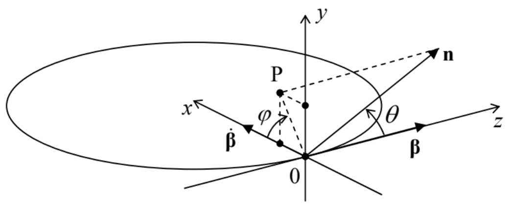Fig. 10.5. The synchrotron radiation problem’s geometry.

In the general case, when the unit vector n toward the radiation’s observer is not within any of the coordinate planes, it has to be described by two angles – the polar angle \(\ \theta\), and the azimuthal angle \(\ \varphi\) between the x-axis and the projection 0P of the vector n to the plane \(\ [x, y]\). Since the length of the segment 0P is \(\ \sin \theta\), the Cartesian components of the relevant vectors are as follows:

\[\ \mathbf{n}=\{\sin \theta \cos \varphi, \sin \theta \sin \varphi, \cos \theta\}, \quad \boldsymbol{\beta}=\{0,0, \beta\}, \quad \text { and } \dot{\boldsymbol{\beta}}=\{\dot{\beta}, 0,0\}.\tag{10.46}\]

Plugging these expressions into the general Eq. (30), we get

\[\ \text{Synchrotron radiation: angular distribution}\quad\quad\quad\quad \begin{gathered}
\frac{d \mathscr{P}}{d \Omega}=\frac{2 Z_{0} q^{2}}{\pi^{2}}|\dot{\boldsymbol{\beta}}|^{2} \gamma^{6} f(\theta, \varphi), \quad \text { where } \\
f(\theta, \varphi) \equiv \frac{1}{8 \gamma^{6}(1-\beta \cos \theta)^{3}}\left[1-\frac{\sin ^{2} \theta \cos ^{2} \varphi}{\gamma^{2}(1-\beta \cos \theta)^{2}}\right]
\end{gathered},\tag{10.47}\]

According to this result, just as at the linear acceleration, in the ultra-relativistic limit, most radiation goes into a narrow cone (of a width \(\ \Delta \theta \sim \gamma^{-1}<<1\)) around the vector \(\ \boldsymbol{\beta}\), i.e. around the instant direction of particle’s propagation. For such small angles, and \(\ \gamma >> 1\),

\[\ f(\theta, \varphi) \approx \frac{1}{\left(1+\gamma^{2} \theta^{2}\right)^{3}}\left[1-\frac{4 \gamma^{2} \theta^{2} \cos ^{2} \varphi}{\left(1+\gamma^{2} \theta^{2}\right)^{2}}\right].\tag{10.48}\]

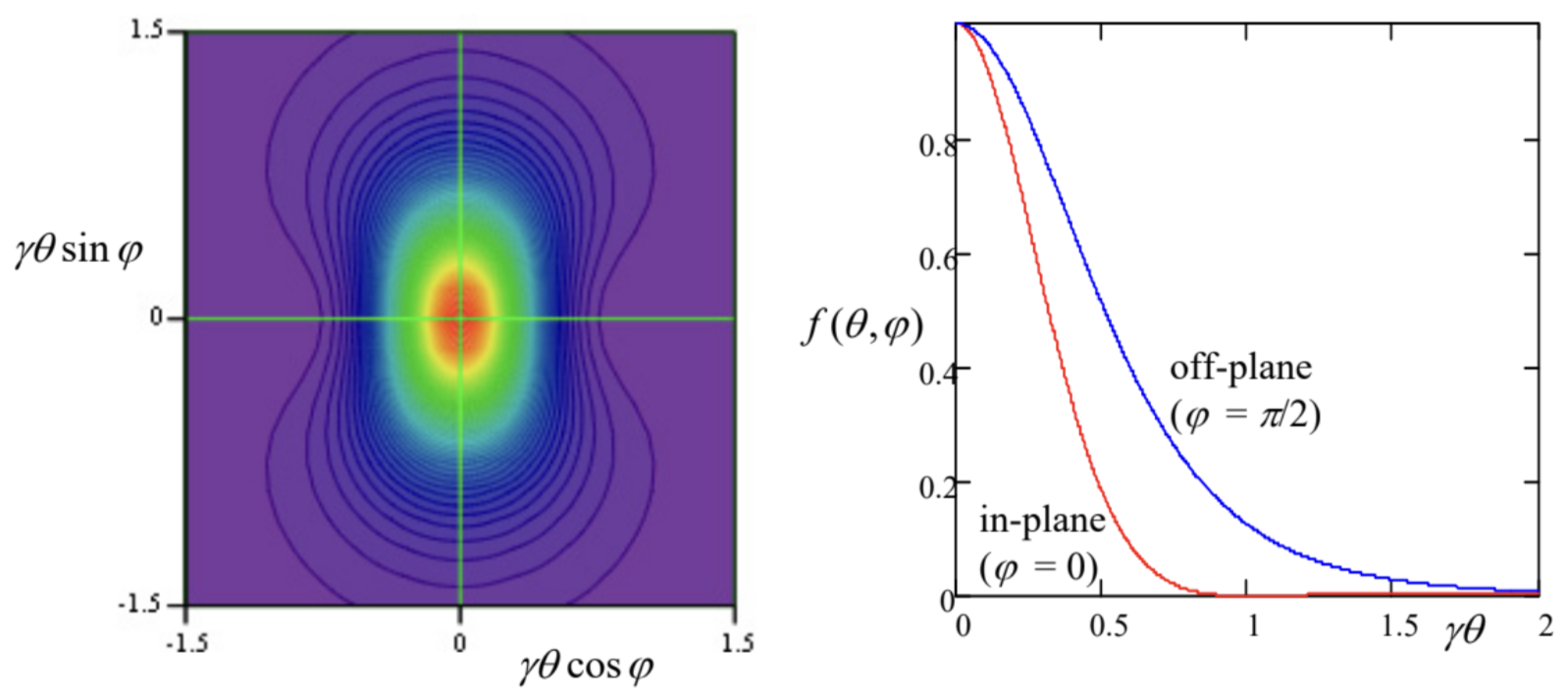
The left panel of Fig. 6 shows a color-coded contour map of this angular distribution \(\ f(\theta, \varphi)\), as observed on a distant plane normal to the particle’s instant velocity (in Fig. 5, parallel to the plane \(\ [x, y]\)), while its right panel shows the factor \(\ f\) as a function of \(\ \theta\) in two perpendicular directions: within the particle’s
rotation plane (in the direction parallel to the x-axis, i.e. at \(\ \varphi=0\)) and perpendicular to this plane (along the y-axis, i.e. at \(\ \varphi=\pm \pi / 2\)). The result shows, first of all, that, in contrast to the case of linear acceleration, the narrow radiation cone is now not hollow: the intensity maximum is reached at \(\ \theta=0\), i.e. exactly in the direction of the particle’s motion direction. Second, the radiation cone is not axially symmetric: within the particle rotation plane, the intensity drops faster (and even has nodes at \(\ \theta=\pm 1 / \gamma\)).

Fig. 10.6. The angular distribution of the synchrotron radiation at \(\ \gamma >> 1\).

As Fig. 5 shows, the angular distribution (47) of the synchrotron radiation was calculated for the (inertial) reference frame whose origin coincides with the particle’s position at this particular instant, i.e. its radiation pattern is time-independent in the frame moving with the particle. This pattern enables a semi-quantitative description of the radiation by an ultra-relativistic particle from the point of view of a stationary observer: if the observation point is on (or very close to) the rotation plane,¹¹ it is being “struck” by the narrow radiation cone once each rotation period \(\ \mathcal{T} \approx 2 \pi R / c\), each “strike” giving a field pulse of a short duration \(\ \Delta t_{\mathrm{ret}}<<1 / \omega_{\mathrm{c}}\) - see Fig. 7.¹²

Fig. 10.7. (a) The synchrotron radiation cones (at \(\ \gamma >> 1\)) for two close values of \(\ t_{\mathrm{ret}}\), and (b) the in-plane component of the electric field, observed in the rotation plane, as a function of time \(\ t\) – schematically.

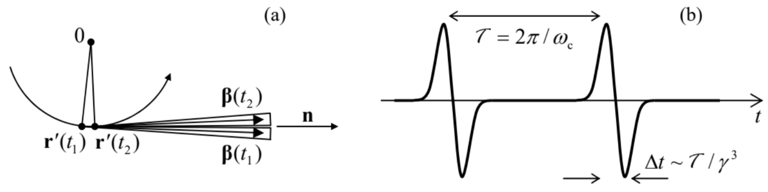
The evaluation of the time duration \(\ \Delta t\) of each pulse requires some care: its estimate \(\ \Delta t_{\mathrm{ret}} \sim 1 / \gamma \omega_{\mathrm{c}}\) is correct for the duration of the retarded time interval during that its cone is aimed at the observer. However, due to the time compression effect discussed in detail in Sec. 1 and described by Eq. (16), the pulse duration as seen by the observer is a factor of \(\ 1 /(1-\beta)\) shorter, so that

\[\ \Delta t=(1-\beta) \Delta t_{\mathrm{ret}} \sim \frac{1-\beta}{\gamma \omega_{\mathrm{c}}} \sim \frac{1}{\gamma^{3} \omega_{\mathrm{c}}} \sim \gamma^{-3} \mathcal{T}, \quad \text { for } \gamma>>1.\tag{10.49}\]

From the Fourier theorem, we can expect the frequency spectrum of such radiation to consist of numerous \(\ \left(N \sim \gamma^{3} >> 1\right)\) harmonics of the particle rotation frequency \(\ \omega_{\mathrm{c}}\), with comparable amplitudes. However, if the orbital frequency fluctuates even slightly \(\ \left(\delta \omega_{\mathrm{c}} / \omega_{\mathrm{c}}>1 / N \sim 1 / \gamma^{3}\right)\), as it happens in most practical systems, the radiation pulses are not coherent, so that the average radiation power spectrum may be calculated as that of one pulse, multiplied by the number of pulses per second. In this case, the spectrum is continuous, extending from low frequencies all the way to approximately

\[\ \omega_{\max } \sim 1 / \Delta t \sim \gamma^{3} \omega_{\mathrm{c}}.\tag{10.50}\]

In order to verify and quantify this result, let us calculate the spectrum of radiation, due to a single pulse. For that, we should first make the general notion of the radiation spectrum quantitative. Let us represent an arbitrary electric field (say that of the synchrotron radiation we are studying now), observed at a fixed point r, as a function of the observation time \(\ t\), as a Fourier integral:¹³

\[\ \mathbf{E}(t)=\int_{-\infty}^{+\infty} \mathbf{E}_{\omega} e^{-i \omega t} d t.\tag{10.51}\]

This expression may be plugged into the formula for the total energy of the radiation pulse (i.e. of the loss of particle’s energy \(\ \mathscr{E}\)) per unit solid angle:¹⁴

\[\ -\frac{d \mathscr{E}}{d \Omega} \equiv \int_{-\infty}^{+\infty} S_{n}(t) R^{2} d t=\frac{R^{2}}{Z_{0}} \int_{-\infty}^{+\infty}|\mathbf{E}(t)|^{2} d t.\tag{10.52}\]

This substitution, followed by a natural change of the integration order, yield

\[\ -\frac{d \mathscr{E}}{d \Omega}=\frac{R^{2}}{Z_{0}} \int_{-\omega}^{+\omega} d \omega \int_{-\omega}^{+\omega} d \omega^{\prime} \mathbf{E}_{\omega} \cdot \mathbf{E}_{\omega^{\prime}} \int_{-\infty}^{+\infty} d t e^{-i\left(\omega+\omega^{\prime}\right) t}.\tag{10.53}\]

But the inner integral (over \(\ t\)) is just \(\ 2 \pi \delta\left(\omega+\omega^{\prime}\right)\).¹⁵ This delta function kills one of the frequency integrals (say, one over \(\ \omega’\)), and Eq. (53) gives us a result that may be recast as

\[\ -\frac{d \mathscr{E}}{d \Omega}=\int_{0}^{+\infty} I(\omega) d \omega, \quad \text { with } I(\omega) \equiv \frac{4 \pi R^{2}}{Z_{0}} \mathbf{E}_{\omega} \cdot \mathbf{E}_{-\omega} \equiv \frac{4 \pi R^{2}}{Z_{0}} \mathbf{E}_{\omega} \mathbf{E}_{\omega}^{*},\tag{10.54}\]

where the evident frequency symmetry of the scalar product \(\ \mathbf{E}_{\omega} \cdot \mathbf{E}_{-\omega}\) has been utilized to fold the integral of \(\ I(\omega)\) to positive frequencies only. The first of Eqs. (54) makes the physical sense of the function \(\ I(\omega)\) very clear: this is the so-called spectral density of the electromagnetic radiation (per unit solid angle).¹⁶

To calculate the spectral density, we can express the function \(\ \mathbf{E}_{\omega}\) via \(\ \mathbf{E}(t)\) using the Fourier transform reciprocal to Eq. (51):

\[\ \mathbf{E}_{\omega}=\frac{1}{2 \pi} \int_{-\infty}^{+\infty} \mathbf{E}(t) e^{i \omega t} d t.\tag{10.55}\]

In the particular case of radiation by a single point charge, we may use here the second (radiative) term of Eq. (19):

\[\ \mathbf{E}_{\omega}=\frac{1}{2 \pi} \frac{q}{4 \pi \varepsilon_{0}} \frac{1}{c R} \int_{-\infty}^{+\infty}\left[\frac{\mathbf{n} \times\{(\mathbf{n}-\boldsymbol{\beta}) \times \dot{\boldsymbol{\beta}}\}}{(1-\boldsymbol{\beta} \cdot \mathbf{n})^{3}}\right]_{\mathrm{ret}} e^{i \omega t} d t.\tag{10.56}\]

Since the vectors n and \(\ \boldsymbol{\beta}\) are more natural functions of the radiation (retarded) time \(\ t_{\mathrm{ret}}\), let us use Eqs. (5) and (16) to exclude the observation time \(\ t\) from this integral:

\[\ \mathbf{E}_{\omega}=\frac{q}{4 \pi \varepsilon_{0}} \frac{1}{2 \pi} \frac{1}{c R} \int_{-\infty}^{+\infty}\left[\frac{\mathbf{n} \times\{(\mathbf{n}-\boldsymbol{\beta}) \times \dot{\boldsymbol{\beta}}\}}{(1-\boldsymbol{\beta} \cdot \mathbf{n})^{2}}\right]_{\mathrm{ret}} \exp \left\{i \omega\left(t_{\mathrm{ret}}+\frac{R_{\mathrm{ret}}}{c}\right)\right\} d t_{\mathrm{ret}}.\tag{10.57}\]

Assuming that the observer is sufficiently far from the particle,¹⁷ we may treat the unit vector n as a constant and also use the approximation (8.19) to reduce Eq. (57) to

\[\ \mathbf{E}_{\omega}=\frac{1}{2 \pi} \frac{q}{4 \pi \varepsilon_{0}} \frac{1}{c R} \exp \left\{\frac{i \omega r}{c}\right\} \int_{-\infty}^{+\infty}\left[\frac{\mathbf{n} \times\{(\mathbf{n}-\boldsymbol{\beta}) \times \dot{\boldsymbol{\beta}}\}}{(1-\boldsymbol{\beta} \cdot \mathbf{n})^{2}} \exp \left\{i \omega\left(t-\frac{\mathbf{n} \cdot \mathbf{r}^{\prime}}{c}\right)\right\}\right]_{\mathrm{ret}} d t_{\mathrm{ret}}.\tag{10.58}\]

Plugging this expression into Eq. (54), and then using the definitions \(\ c \equiv 1 /\left(\varepsilon_{0} \mu_{0}\right)^{1 / 2}\) and \(\ Z_{0} \equiv\left(\mu_{0} / \varepsilon_{0}\right)^{1 / 2}\), we get¹⁸

\[\ I(\omega)=\frac{Z_{0} q^{2}}{16 \pi^{3}}\left|\int_{-\infty}^{+\infty}\left[\frac{\mathbf{n} \times\{(\mathbf{n}-\boldsymbol{\beta}) \times \dot{\boldsymbol{\beta}}\}}{(1-\boldsymbol{\beta} \cdot \mathbf{n})^{2}} \exp \left\{i \omega\left(t-\frac{\mathbf{n} \cdot \mathbf{r}^{\prime}}{c}\right)\right\}\right]_{\mathrm{ret}} d t_{\mathrm{ret}}\right|^{2}.\tag{10.59}\]

This result may be further simplified by noticing that the fraction before the exponent may be represented as a full derivative over \(\ t_{\mathrm{ret}}\),

\[\ \left[\frac{\mathbf{n} \times\{(\mathbf{n}-\boldsymbol{\beta}) \times \dot{\boldsymbol{\beta}}\}}{(1-\boldsymbol{\beta} \cdot \mathbf{n})^{2}}\right]_{\mathrm{ret}} \equiv\left[\frac{\mathbf{n} \times\{(\mathbf{n}-\boldsymbol{\beta}) \times d \boldsymbol{\beta} / d t\}}{(1-\boldsymbol{\beta} \cdot \mathbf{n})^{2}}\right]_{\mathrm{ret}} \equiv \frac{d}{d t}\left[\frac{\mathbf{n} \times(\mathbf{n} \times \boldsymbol{\beta})}{1-\boldsymbol{\beta} \cdot \mathbf{n}}\right]_{\mathrm{ret}},\tag{10.60}\]

and working out the resulting integral by parts. At this operation, the time differentiation of the parentheses in the exponent gives \(\ d\left[t_{\mathrm{ret}}-\mathbf{n} \cdot \mathbf{r}^{\prime}\left(t_{\mathrm{ret}}\right) / c\right] / d t_{\mathrm{ret}}=(1-\mathbf{n} \cdot \mathbf{u} / c)_{\mathrm{ret}} \equiv(1-\boldsymbol{\beta} \cdot \mathbf{n})_{\mathrm{ret}}\), leading to the cancellation of the remaining factor in the denominator and hence to a very simple general result:¹⁹

\[\ \text{Relativistic radiation: spectral density}\quad\quad\quad\quad I(\omega)=\frac{Z_{0} q^{2} \omega^{2}}{16 \pi^{3}}\left|\int_{-\infty}^{+\infty}\left[\mathbf{n} \times(\mathbf{n} \times \boldsymbol{\beta}) \exp \left\{i \omega\left(t-\frac{\mathbf{n} \cdot \mathbf{r}^{\prime}}{c}\right)\right\}\right]_{\mathrm{ret}} d t_{\mathrm{ret}}\right|^{2}.\tag{10.61}\]

Now returning to the particular case of the synchrotron radiation, it is beneficial to choose the origin of time \(\ t_{\mathrm{ret}}\) so that at \(\ t_{\mathrm{ret}}=0\), the angle \(\ \theta\) between the vectors n and \(\ \boldsymbol{\beta}\) takes its smallest value \(\ \theta_{0}\), i.e., in terms of Fig. 5, the vector n is within the plane \(\ [y, z]\). Fixing this direction of the axes, so that they do not move in further times, we can redraw that figure as shown in Fig. 8.

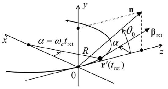
Fig. 10.8. Deriving the synchrotron radiation’s spectral density. The vector n is static within the plane \(\ [y, z]\), while the vectors \(\ \mathbf{r}^{\prime}\left(t_{\mathrm{ret}}\right)\) and \(\ \boldsymbol{\beta}_{\text {ret }}\) rotate, within the plane \(\ \left[\begin{array}{ll}
x, & z
\end{array}\right]\), with the angular velocity \(\ \omega_{c}\) of the particle.

In this “lab” reference frame, the vector n does not depend on time, while the vectors \(\ \mathbf{r}^{\prime}\left(t_{\mathrm{ret}}\right)\) and \(\ \boldsymbol{\beta}_{\mathrm{ret}}\) do depend on it via the angle \(\ \alpha \equiv \omega_{\mathrm{c}} t_{\mathrm{ret}}\):,

\[\ \mathbf{n}=\left\{0, \sin \theta_{0}, \cos \theta_{0}\right\}, \quad \mathbf{r}^{\prime}\left(t_{\mathrm{ret}}\right)=\{R(1-\cos \alpha), 0, R \sin \alpha\}, \quad \boldsymbol{\beta}_{\mathrm{ret}} \equiv\{\beta \sin \alpha, 0, \beta \cos \alpha\}.\tag{10.62}\]

Now an easy multiplication yields

\[\ [\mathbf{n} \times(\mathbf{n} \times \boldsymbol{\beta})]_{\mathrm{ret}}=\beta\left\{\sin \alpha, \sin \theta_{0} \cos \theta_{0} \cos \alpha,-\sin ^{2} \theta_{0} \sin \alpha\right\},\tag{10.63}\]

\[\ \left[\exp \left\{i \omega\left(t-\frac{\mathbf{n} \cdot \mathbf{r}^{\prime}}{c}\right)\right\}\right]_{\mathrm{ret}}=\exp \left\{i \omega\left(t_{\mathrm{ret}}-\frac{R}{c} \cos \theta_{0} \sin \alpha\right)\right\}.\tag{10.64}\]

As we already know, in the (most interesting) ultra-relativistic limit \(\ \gamma >> 1\), most radiation is confined to short pulses, so that only small angles \(\ \alpha \sim \omega_{\mathrm{c}} \Delta t_{\mathrm{ret}} \sim \gamma^{-1}\) may contribute to the integral in Eq. (61). Moreover, since most radiation goes to small angles \(\ \theta \sim \theta_{0} \sim \gamma^{-1}\), it makes sense to consider only such small angles. Expanding both trigonometric functions of these small angles, participating in parentheses of Eq. (64), into the Taylor series, and keeping only the leading terms, we get

\[\ t_{\mathrm{ret}}-\frac{R}{c} \cos \theta_{0} \sin \alpha \approx t_{\mathrm{ret}}-\frac{R}{c} \omega_{\mathrm{c}} t_{\mathrm{ret}}+\frac{R}{c} \frac{\theta_{0}^{2}}{2} \omega_{\mathrm{c}} t_{\mathrm{ret}}+\frac{R}{c} \frac{\omega_{\mathrm{c}}^{3}}{6} t_{\mathrm{ret}}^{3}.\tag{10.65}\]

Since \(\ (R / c) \omega_{\mathrm{c}}=u / c=\beta \approx 1\), in the two last terms we may approximate this parameter by 1. However, it is crucial to distinguish the difference of the two first terms, proportional to \(\ (1-\beta) t_{\mathrm{ret}}\), from zero; as we have done before, we may approximate it with \(\ t_{\mathrm{ret}} / 2 \gamma^{2}\). On the right-hand side of Eq. (63), which does not have such a critical difference, we may be bolder, taking²⁰

\[\ \beta\left\{\sin \alpha, \sin \theta_{0} \cos \theta_{0} \cos \alpha,-\sin ^{2} \theta_{0} \sin \alpha\right\} \approx\left\{\alpha, \theta_{0}, 0\right\} \equiv\left\{\omega_{\mathrm{c}} t_{\mathrm{ret}}, \theta_{0}, 0\right\}.\tag{10.66}\]

As a result, Eq. (61) is reduced to

\[\ I(\omega)=\frac{Z_{0} q^{2}}{16 \pi^{3}}\left|a_{x} \mathbf{n}_{x}+a_{y} \mathbf{n}_{y}\right|^{2} \equiv \frac{Z_{0} q^{2}}{16 \pi^{3}}\left(\left|a_{x}\right|^{2}+\left|a_{y}\right|^{2}\right),\tag{10.67}\]

where \(\ a_{x}\) and \(\ a_{y}\) are the following dimensionless factors:

Synchrotron radiation: spectral density

\[\ \begin{aligned}
&a_{x} \equiv \omega \int_{-\infty}^{+\infty} \omega_{\mathrm{c}} t_{\mathrm{ret}} \exp \left\{\frac{i \omega}{2}\left(\left(\theta_{0}^{2}+\gamma^{-2}\right) t_{\mathrm{ret}}+\frac{\omega_{\mathrm{c}}^{2}}{3} t_{\mathrm{ret}}^{3}\right)\right\} d t_{\mathrm{ret}}, \\
&a_{y} \equiv \omega \int_{-\infty}^{+\infty} \theta_{0} \exp \left\{\frac{i \omega}{2}\left(\left(\theta_{0}^{2}+\gamma^{-2}\right) t_{\mathrm{ret}}+\frac{\omega_{\mathrm{c}}^{2}}{3} t_{\mathrm{ret}}^{3}\right)\right\} d t_{\mathrm{ret}},
\end{aligned}\tag{10.68}\]

that describe the frequency spectra of two components of the synchrotron radiation, with mutually perpendicular directions of polarization. Defining the following dimensionless parameter

\[\ \nu \equiv \frac{\omega}{3 \omega_{\mathrm{c}}}\left(\theta_{0}^{2}+\gamma^{-2}\right)^{3 / 2},\tag{10.69}\]

which is proportional to the observation frequency, and changing the integration variable to \(\ \xi\equiv \omega_{\mathrm{c}} t_{\mathrm{ret}} /\left(\theta_{0}^{2}+\gamma^{-2}\right)^{1 / 2}\), the integrals (68) may be reduced to the modified Bessel functions of the second kind, but with fractional indices:

\[\ \begin{aligned}
&a_{x}=\frac{\omega}{\omega_{c}}\left(\theta_{0}^{2}+\gamma^{-2}\right) \int_{-\infty}^{+\infty} \xi \exp \left\{\frac{3}{2} i \nu\left(\xi+\frac{\xi^{3}}{3}\right)\right\} d \xi=\frac{2 \sqrt{3} i}{\left(\theta_{0}^{2}+\gamma^{-2}\right)^{1 / 2}} \nu K_{2 / 3}(\nu) \\
&a_{y}=\frac{\omega}{\omega_{c}} \theta_{0}\left(\theta_{0}^{2}+\gamma^{-2}\right)^{1 / 2} \int_{-\infty}^{+\infty} \exp \left\{\frac{3}{2} i \nu\left(\xi+\frac{\xi^{3}}{3}\right)\right\} d \xi=\frac{2 \sqrt{3} \theta_{0}}{\theta_{0}^{2}+\gamma^{-2}} \nu K_{1 / 3}(\nu)
\end{aligned}\tag{10.70}\]

Figure 9a shows the dependence of the Bessel factors, defining the amplitudes ax and ay, on the normalized observation frequency \(\ \nu\). It shows that the radiation intensity changes with frequency relatively slowly (note the log-log scale of the plot!) until the normalized frequency, defined by Eq. (69), is increased beyond ~1. For most important observation angles \(\ \theta_{0} \sim \gamma\) this means that our estimate (50) is indeed correct, though formally the frequency spectrum extends to infinity.²¹

Fig. 10.9. The frequency spectra of: (a) two components of the synchrotron radiation, at a fixed angle \(\ \theta_{0}\), and (b) its total (polarization- and angle-averaged) intensity.

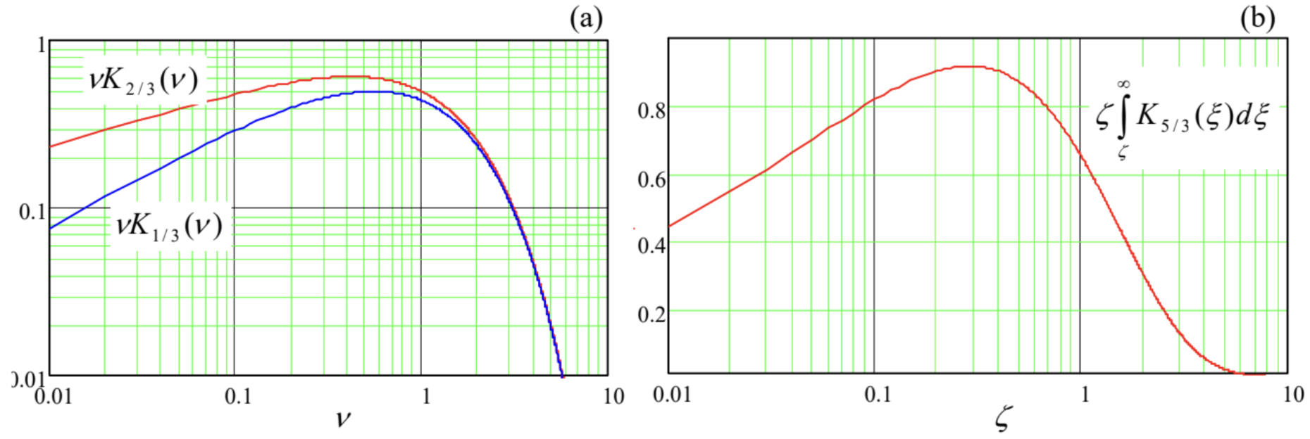
Naturally, the spectral density integrated over the full solid angle exhibits a similar frequency behavior. Without performing the integration,²² let me just give the result (also valid for \(\ \gamma>>1\) only) for the reader’s reference:

\[\ \oint_{4 \pi} I(\omega) d \Omega=\frac{\sqrt{3}}{4 \pi} q^{2} \gamma \zeta \int_{\zeta}^{\infty} K_{5 / 3}(\xi) d \xi, \quad \text { where } \zeta \equiv \frac{2}{3} \frac{\omega}{\omega_{c} \gamma^{3}}.\tag{10.71}\]

Figure 9b shows the dependence of this integral on the normalized frequency \(\ \zeta\). (This plot is sometimes called the “universal flux curve”.) In accordance with the estimate (50), it reaches the maximum at

\[\ \zeta_{\max } \approx 0.3, \quad \text { i.e. } \omega_{\max } \approx \frac{\omega_{\mathrm{c}}}{2} \gamma^{3}.\tag{10.73}\]

For example, in the National Synchrotron Light Source (NSLS-II) in the Brookhaven National Laboratory, near the SBU campus, with the ring circumference of 792 m, the electron revolution period \(\ \mathcal{T}\) is 2.64 μs. Calculating \(\ \omega_{\mathrm{c}}\) as \(\ 2 \pi / \mathcal{T} \approx 2.4 \times 10^{6} \mathrm{~s}^{-1}\), for the achieved \(\ \gamma \approx 6 \times 10^{3}(\mathscr{E} \approx 3 \mathrm{GeV})\), we get \(\ \omega_{\max }\sim 3\times10^{17}s^{-1}\) (the photon energy \(\ \hbar \omega_{\max } \sim 200 \mathrm{eV}\)), corresponding to soft X-rays. In the light of this estimate, the reader may be surprised by Fig. 10, which shows the calculated spectra of the radiation that this facility was designed to produce, with the intensity maxima at photon energies up to a few keV.

Fig. 10.10. Design brightness of various synchrotron radiation sources of the NSLS-II facility. For bend magnets and wigglers, the “brightness” may be obtained by multiplication of the spectral density \(\ I(\omega)\) from one electron pulse, calculated above, by the number of electrons passing the source per second. (Note the non-SI units used by the synchrotron radiation community.) However, for undulators, there is an additional factor due to the partial coherence of radiation – see below. (Adapted from NSLS-II Source Properties and Floor Layout, was available online at https://www.bnl.gov/ps/docs/pdf/SourceProperties.pdf in 2011-2010.)

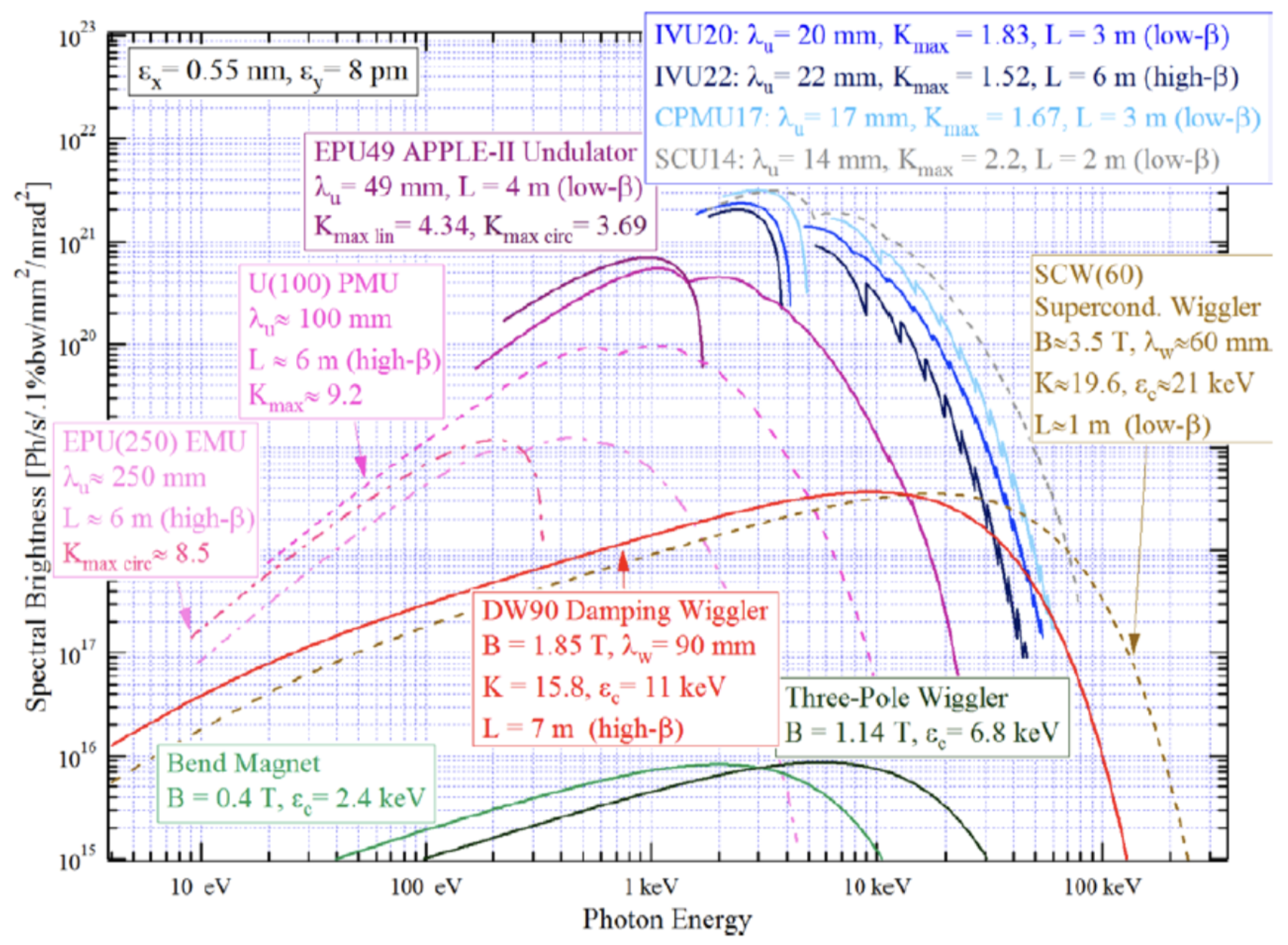
The reason for this discrepancy is that in the NLLS-II, and in all modern synchrotron light sources, most radiation is produced not by the circular orbit itself (which is, by the way, not exactly circular, but consists of a series of straight and bend-magnet sections), but by such bend sections, and the devices called wigglers and undulators: strings of several strong magnets with alternating field direction (Fig. 11), that induce periodic bending (wiggling”) of the electron’s trajectory, with the synchrotron radiation emitted at each bend.

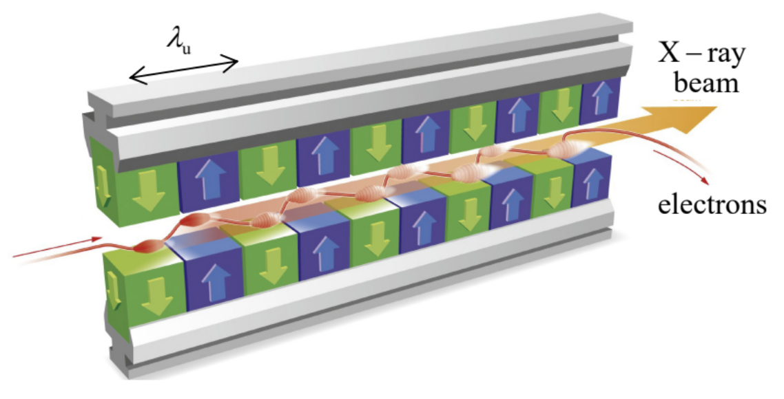Fig. 10.11. The generic structure of the wigglers, undulators, and free-electron lasers. (Adapted from http://www.xfel.eu/overview/how_does_it_work/. )

The difference between the wigglers and the undulators is more quantitative than qualitative: the former devices have a larger spatial period \(\ \lambda_{\mathrm{u}}\) (the distance between the adjacent magnets of the same polarity, see Fig. 11), giving enough space for the electron beam to bend by an angle larger than \(\ \gamma^{-1}\), i.e.
larger than the radiation cone’s width. As a result, the radiation arrives to an in-plane observer as a periodic sequence of individual pulses – see Fig. 12a.

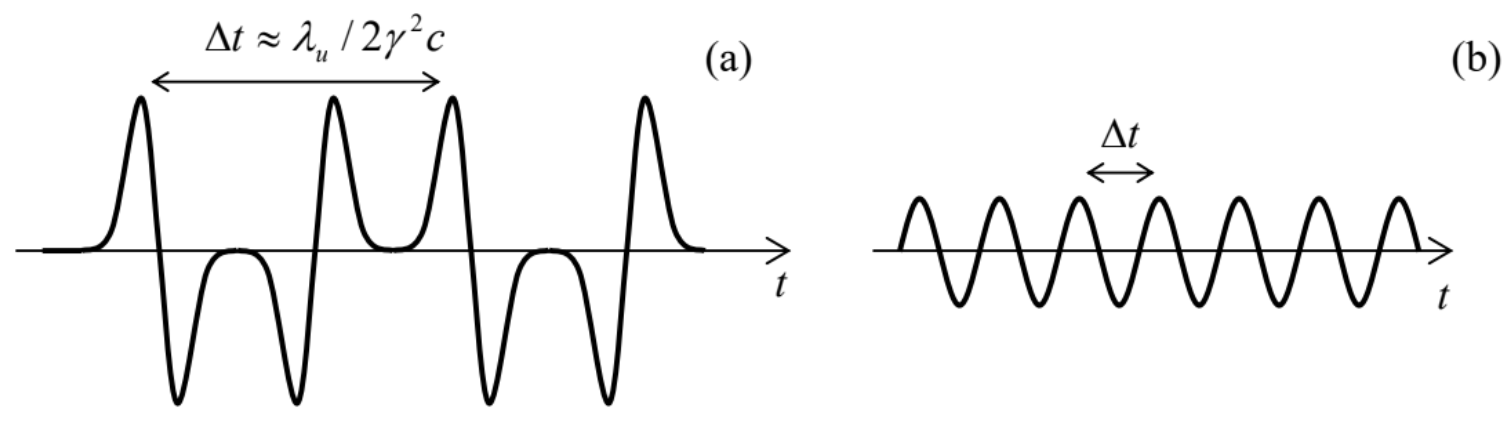Fig. 10.12. Waveforms of the radiation emitted by (a) a wiggler and (b) an undulator – schematically.

The shape of each pulse, and hence its frequency spectrum, are essentially similar to those discussed above,²³ but with much higher local values of \(\ \omega_{\mathrm{c}}\) and hence \(\ \omega_{\max }\) – see Fig. 10. Another difference is a much higher frequency of the pulses. Indeed, the fundamental Eq. (16) allows us to calculate the time distance between them, for the observer, as

\[\ \Delta t \approx \frac{\partial t}{\partial t_{\text {ret }}} \Delta t_{\text {ret }} \approx(1-\beta) \frac{\lambda_{\mathrm{u}}}{u} \approx \frac{1}{2 \gamma^{2}} \frac{\lambda_{\mathrm{u}}}{c}<<\frac{\lambda_{\mathrm{u}}}{c},\tag{10.73}\]

where the first two relations are valid at \(\ \lambda_{\mathrm{u}}<<R\) (the relation typically satisfied very well, see the numbers in Fig. 10), and the last two relations assume the ultra-relativistic limit. As a result, the radiation intensity, which is proportional to the number of the poles, is much higher than that from the bend magnets – see Fig. 10 again.

The situation is different in undulators – similar structures with a smaller spatial period \(\ \lambda_u\), in which the electron’s velocity vector oscillates with an angular amplitude smaller than \(\ \gamma^{-1}\). As a result, the radiation pulses overlap (Fig. 12b) and the radiation waveform is closer to the sinusoidal one. As a result, the radiation spectrum narrows to the central frequency²⁴

\[\ \omega_{0}=\frac{2 \pi}{\Delta t} \approx 2 \gamma^{2} \frac{2 \pi c}{\lambda_{u}}.\tag{10.74}\]

For example, for the LSNL-II undulators with \(\ \lambda_{\mathrm{u}}=2 \mathrm{~cm}\), this formula predicts a radiation peak at phonon energy \(\ \hbar \omega_{0} \approx 4 \mathrm{keV}\), in a reasonable agreement with the results of quantitative calculations, shown in Fig. 10.²⁵ Due to the spectrum narrowing, the intensity of undulator’s radiation is higher than that of wigglers using the same electron beam.

This spectrum-narrowing trend is brought to its logical conclusion in the so-called free-electron lasers²⁶ whose basic structure is the same as that of wigglers and undulators (Fig. 11), but the radiation at each beam bend is so intense and narrow-focused that it affects the electron motion downstream the radiation cone. As a result, the radiation spectrum narrows around the central frequency (74), and its power grows as a square of the number N of electrons in the structure (rather than proportionately to N in wigglers and undulators).

Finally, note that wigglers, undulators, and free-electron lasers may be also used at the end of a linear electron accelerator (such as SLAC) which, as was noted above, may provide extremely high values of \(\ \gamma\), and hence radiation frequencies, due to the smallness of radiation energy losses at the electron acceleration stage. Very unfortunately, I do not have time/space to discuss (very interesting) physics of these devices in more detail.²⁷

---

Reference

¹¹ It is easy (and hence is left for the reader’s exercise) to show that if the observation point is much off-plane (say, is located on the particle orbit’s axis), the radiation is virtually monochromatic, with frequency \(\ \omega_{c}\). (As we know from Sec. 8.2, in the non-relativistic limit \(\ u<<c\) this is true for any observation point.)

¹² The fact that the in-plane component of each electric field’s pulse \(\ \mathbf{E}(t)\) is antisymmetric with respect to its central point, and hence vanishes at that point (as Fig. 7b shows), readily follows from Eq. (19).

¹³ In contrast to the single-frequency case (i.e. a monochromatic wave), we may avoid taking the real part of the complex function \(\ \left(\mathbf{E}_{\omega} e^{-i \omega t}\right)\) by requiring that in Eq. (51), \(\ \mathbf{E}_{-\omega}=\mathbf{E}_{\omega}^{*}\). However, it is important to remember the factor 1⁄2 required for the transition to a monochromatic wave of frequency \(\ \omega_{0}\) and with real amplitude \(\ \mathbf{E}_{0}\): \(\ \mathbf{E}_{\omega}=\mathbf{E}_{0}\left[\delta\left(\omega-\omega_{0}\right)+\delta\left(\omega+\omega_{0}\right)\right] / 2\)

¹⁴ Note that the expression under this integral differs from \(\ d \mathscr{P} / d \Omega\) defined by Eq. (29) by the absence of the term \(\ (1-\boldsymbol{\beta} \cdot \mathbf{n})=\partial t_{\mathrm{ret}} / \partial t\) – see Eq. (16). This is natural because now we are calculating the wave energy arriving at the observation point r during the time interval \(\ dt\) rather than \(\ d t_{\mathrm{ret}}\).

¹⁵ See, e.g. MA Eq. (14.4).

¹⁶ The notion of spectral density may be readily generalized to random processes – see, e.g., SM Sec. 5.4.

¹⁷ According to the estimate (49), for a synchrotron radiation’s pulse, this restriction requires the observer to be much farther than \(\ \Delta r^{\prime} \sim c \Delta t \sim R / \gamma^{3}\) from the particle. With the values \(\ R \sim 10^{4}\) and \(\ \gamma \sim 10^{5}\) mentioned above, \(\ \Delta r^{\prime} \sim10^{-11}\mathrm{m}\), so this requirement is satisfied for any realistic radiation detector.

¹⁸ Note that for our current purposes of calculation of the spectral density of radiation by a single particle, the factor \(\ \exp \{i \omega r / c\}\) has got canceled. However, as we have seen in Chapter 8, this factor plays the central role at the interference of radiation from several (many) sources. Such interference is important, in particular, in undulators and free-electron lasers – the devices to be (qualitatively) discussed below.

¹⁹ Actually, this simplification is not occasional. According to Eq. (10b), the expression under the derivative in the last form of Eq. (60) is just the transverse component of the vector potential \(\ \boldsymbol{A}\) (give or take a constant factor), and from the discussion in Sec. 8.2 we know that this component determines the electric dipole radiation of the particle, which dominates the radiation field in our current case of a particle with a non-zero electric charge.

²⁰ This expression confirms that the in-plane (x) component of the electric field is an odd function of \(\ t_{\mathrm{ret}}\) and hence of \(\ t-t_{0}\) (see its sketch in Fig. 7b), while the normal \(\ (y)\) component is an even function of this difference. Also, note that for an observer exactly in the rotation plane \(\ \left(\theta_{0}=0\right)\) the latter component equals zero for all times – the fact which could be predicted from the very beginning because of the evident mirror symmetry of the problem with respect to the particle rotation plane.

²¹ The law of the spectral density decrease at large \(\ \nu\) may be readily obtained from the second of Eqs. (2.158), which is valid even for any (even non-integer) Bessel function index \(\ n\): \(\ a_{x} \propto a_{y} \propto \nu^{-1 / 2} \exp \{-\nu\}\). Here the exponential factor is certainly the most important one.

²² For that, and many other details, the interested reader may be referred, for example, to the fundamental review collection by E. Koch et al. (eds.) Handbook on Synchrotron Radiation (in 5 vols.), North-Holland, 1983-1991, or to a more concise monograph by A. Hofmann, The Physics of Synchrotron Radiation, Cambridge U. Press, 2007.

²³ Indeed, the period \(\ \lambda_{u}\) is typically a few centimeters (see the numbers in Fig. 10), i.e. is much larger than the interval \(\ \Delta r^{\prime} \sim R / \gamma^{3}\) estimated above. Hence the synchrotron radiation results may be applied locally, to each electron beam’s bend. (In this context, a simple problem for the reader: use Eqs. (19) and (63) to explain the difference between shapes of the in-plane electric field pulses emitted at opposite magnetic poles of the wiggler, which is schematically shown in Fig. 12a.)

²⁴ This important formula may be also derived in the following way. Due to the relativistic length contraction (9.20), the undulator structure period as perceived by beam electrons is \(\ \lambda^{\prime}=\lambda_{u} / \gamma\), so that the central frequency of the radiation in the reference frame moving with the electrons is \(\ \omega_{0}^{\prime}=2 \pi c / \lambda^{\prime}=2 \pi c \gamma / \lambda_{u}\). For the lab-frame observer, this frequency is Doppler-upshifted in accordance with Eq. (9.44): \(\ \omega_{0}=\omega_{0}{ }^{\prime}[(1+\beta) /(1-\beta)]^{1 / 2} \approx 2 \gamma \omega_{0}’\), giving the same result as Eq. (74).

²⁵ Some of the difference is due to the fact that those plots show the spectral density of the number of photons \(\ n=\mathscr{E}/\hbar\omega\) per second, which peaks at a frequency below that of the density of power, i.e. of the energy \(\ \mathscr{E}\) per second.

²⁶ This name is somewhat misleading, because in contrast to the usual (“quantum”) lasers, a free-electron laser is essentially a classical device, and the dynamics of electrons in it is very similar to that in vacuum-tube microwave generators, such as the magnetrons briefly discussed in Sec. 9.6.

²⁷ The interested reader may be referred, for example, to either P. Luchini and H. Motz, Undulators and Free-electron Lasers, Oxford U. Press, 1990; or E. Salin et al., The Physics of Free Electron Lasers, Springer, 2000.