10.2: Radiation Power

Let us calculate the angular distribution of the particle’s radiation. For that, we need to return to Eqs. (19)-(20) to find the Poynting vector \(\ \mathbf{S}=\mathbf{E} \times \mathbf{H}\), and in particular its radial component \(\ S_{n}=\mathbf{S} \cdot \mathbf{n}_{\mathrm{ret}}\), at large distances \(\ R\) from the particle. Following tradition,⁷ let us express the result as the energy radiated into unit solid angle per unit time interval \(\ d t_{\mathrm{rad}}\) of the radiation, rather than that (\(\ dt\)) of its measurement. (We will need to return to the measurement time \(\ t\) in the next section, to calculate the observed radiation spectrum.) Using Eq. (16), we get

\[\ \frac{d \mathscr{P}}{d \Omega} \equiv-\frac{d \mathscr{E}}{d \Omega d t_{\mathrm{ret}}}=\left(R^{2} S_{n}\right)_{\mathrm{ret}} \frac{\partial t}{\partial t_{\mathrm{ret}}}=(\mathbf{E} \times \mathbf{H}) \cdot\left[R^{2} \mathbf{n}(1-\boldsymbol{\beta} \cdot \mathbf{n})\right]_{\mathrm{ret}}.\tag{10.29}\]

At sufficiently large distances from the particle, i.e. in the limit \(\ R_{\mathrm{ret}} \rightarrow \infty\) (in the radiation zone), the contribution of the first (essentially, the Coulomb-field) term in the square brackets of Eq. (19) vanishes as \(\ 1 / R^{2}\), and the substitution of the remaining term into Eqs. (20) and then (29) yields the following formula, valid for an arbitrary law of particle motion:⁸

\[\ \text{Radiation power density}\quad\quad\quad\quad \frac{d \mathscr{P}}{d \Omega}=\frac{Z_{0} q^{2}}{(4 \pi)^{2}} \frac{|\mathbf{n} \times[(\mathbf{n}-\boldsymbol{\beta}) \times \dot{\boldsymbol{\beta}}]|^{2}}{(1-\mathbf{n} \cdot \boldsymbol{\beta})^{5}}.\tag{10.30}\]

Now, let us apply this important result to some simple cases. First of all, Eq. (30) says that a charge moving with a constant velocity \(\ \boldsymbol{\beta}\) does not radiate at all. This might be expected from our analysis of this case in Sec. 9.5 because in the reference frame moving with the charge it produces only the Coulomb electrostatic field, i.e. no radiation.

Next, let us consider a linear motion of a point charge with a non-zero acceleration – directed along the straight line of the motion. In this case, with the coordinate axes selected shown in Fig. 4a, each of the vectors involved in Eq. (30) has at most two non-zero Cartesian components:

\[\ \mathbf{n}=\{\sin \theta, 0, \cos \theta\}, \quad \boldsymbol{\beta}=\{0,0, \beta\}, \quad \dot{\boldsymbol{\beta}}=\{0,0, \dot{\beta}\},\tag{10.31}\]

where \(\ \theta\) is the angle between the directions of the particle’s motion and of the radiation’s propagation. Plugging these expressions into Eq. (30) and performing the vector multiplications, we readily get

\[\ \frac{d \mathscr{P}}{d \Omega}=\frac{Z_{0} q^{2}}{(4 \pi)^{2}} \dot{\beta}^{2} \frac{\sin ^{2} \theta}{(1-\beta \cos \theta)^{5}}.\tag{10.32}\]

Figure 4b shows the angular distribution of this radiation, for three values of the particle’s speed \(\ u\).

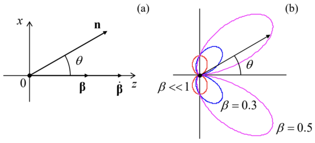Fig. 10.4. Particle’s radiation at linear acceleration: (a) the problem’s geometry, and (b) the last fraction of Eq. (32) as a function of the angle \(\ \theta\).

If the speed is relatively low \(\ (u<<c \text {, i.e. } \beta<<1)\), the denominator in Eq. (32) is very close to 1 for all observation angles \(\ \theta\), so that the angular distribution of the radiation power is close to \(\ \sin ^{2} \theta\) – just as it follows from the general non-relativistic Larmor formula (8.26), for our current case with \(\ \Theta=\theta\). However, as the velocity is increased, the denominator becomes less than 1 for \(\ \theta<\pi / 2\), i.e. for the forward-looking directions, and larger than 1 for back directions. As a result, the radiation in the direction of the particle’s motion is increased (somewhat counter-intuitively, regardless of the acceleration’s sign!), while that in the back direction is suppressed. For ultra-relativistic particles \(\ (\beta \rightarrow 1)\), this trend is strongly exacerbated, and radiation to very small forward angles dominates. To describe this main part of the angular distribution, we may expand the trigonometric functions of \(\ \theta\) participating in Eq. (32) in the Taylor series in small \(\ \theta\), and keep only their leading terms: \(\ \sin \theta \approx \theta, \cos \theta \approx 1-\theta^{2} / 2\), so that \(\ (1-\beta \cos \theta) \approx\left(1+\gamma^{2} \theta^{2}\right) / 2 \gamma^{2}\). The resulting expression,

\[\ \frac{d \mathscr{P}}{d \Omega} \approx \frac{2 Z_{0} q^{2}}{\pi^{2}} \dot{\beta}^{2} \gamma^{8} \frac{(\gamma \theta)^{2}}{\left(1+\gamma^{2} \theta^{2}\right)^{5}}, \quad \text { for } \gamma >> 1,\tag{10.33}\]

describes a narrow “hollow cone” distribution of radiation, with its maximum at the angle

\[\ \theta_{0}=\frac{1}{2 \gamma}<<1.\tag{10.34}\]

Another important aspect of Eq. (33) is how extremely fast (as \(\ \gamma^8\)) the radiation density grows with the Lorentz factor \(\ \gamma\), i.e. with the particle’s energy \(\ \mathscr{E}=\gamma m c^{2}\).

Still, the total radiated power \(\ \mathscr{P}\) (into all observation angles) at linear acceleration is not too high for any practicable values of parameters. To show this, let us first calculate \(\ \mathscr{P}\) for an arbitrary motion of the particle. To start, let me demonstrate how \(\ \mathscr{P}\) may be found (or rather guessed) from the general relativistic arguments. In Sec. 8.2, we have derived Eq. (8.27) for the power of the electric dipole radiation for a non-relativistic particle motion. That result is valid, in particular, for one charged particle, whose electric dipole moment’s derivative over time may be expressed as \(\ d(q \mathbf{r}) / d t=(q / m) \mathbf{p}\), where \(\ \mathbf{p}\) is
the particle’s linear mechanical momentum (not its electric dipole moment). As the result, the Larmor formula (8.27) in free space, i.e. with \(\ \nu=c\) (but \(\ u<<c\)) reduces to

\[\ \mathscr{P}=\frac{Z_{0}}{6 \pi c^{2}}\left(\frac{q}{m} \frac{d p}{d t}\right)^{2} \equiv \frac{Z_{0} q^{2}}{6 \pi m^{2} c^{2}}\left(\frac{d \mathbf{p}}{d t} \cdot \frac{d \mathbf{p}}{d t}\right), \quad \text { for } u<<c.\tag{10.35}\]

This is evidently not a Lorentz-invariant result, but it gives a clear hint of how such an invariant, that would be reduced to Eq. (35) in the non-relativistic limit, may be formed:

\[\ \mathscr{P}=-\frac{Z_{0} q^{2}}{6 \pi m^{2} c^{2}}\left(\frac{d p_{\alpha}}{d \tau} \cdot \frac{d p^{\alpha}}{d \tau}\right) \equiv \frac{Z_{0} q^{2}}{6 \pi m^{2} c^{2}}\left[\left(\frac{d \mathbf{p}}{d \tau}\right)^{2}-\frac{1}{c^{2}}\left(\frac{d \mathscr{E}}{d \tau}\right)^{2}\right].\tag{10.36}\]

Using the relativistic expressions \(\ \mathbf{p}=\gamma m c \boldsymbol{\beta}, \mathscr{E}=\gamma m c^{2}, \text { and } d \tau=d t / \gamma\), the last formula may be recast into the so-called Liénard extension of the Larmor formula:⁹

\[\ \text{Total radiation power via }\beta\quad\quad\quad\quad\mathscr{P}=\frac{Z_{0} q^{2}}{6 \pi} \gamma^{6}\left[(\dot{\boldsymbol{\beta}})^{2}-(\boldsymbol{\beta} \times \dot{\boldsymbol{\beta}})^{2}\right] \equiv \frac{Z_{0} q^{2}}{6 \pi} \gamma^{4}\left[(\dot{\boldsymbol{\beta}})^{2}+\gamma^{2}(\boldsymbol{\beta} \cdot \dot{\boldsymbol{\beta}})^{2}\right].\tag{10.37}\]

It may be also obtained by direct integration of Eq. (30) over the full solid angle, thus confirming our guess.

However, for some applications, it is beneficial to express \(\ \mathscr{P}\) via the time evolution of the particle’s momentum alone. For that, we may differentiate the fundamental relativistic relation (9.78), \(\ \mathscr{E}^{2}=\left(m c^{2}\right)^{2}+(p c)^{2}\), over the proper time \(\ \tau\) to get

\[\ \text{Total radiation power via p}\quad\quad\quad\quad 2\mathscr{E} \frac{d{\mathscr{E}}}{d \tau}=2 c^{2} p \frac{d p}{d \tau}, \quad\quad\quad \text { i.e. } \frac{d \mathscr{E}}{d \tau}=\frac{c^{2} p}{\mathscr{E}} \frac{d p}{d \tau}=u \frac{d p}{d \tau},\tag{10.39}\]

Please note the difference between the squared derivatives in this expression: in the first of them we have to differentiate the momentum vector p first, and only then form a scalar by squaring the resulting vector derivative, while in the second case, only the magnitude of the vector has to be differentiated. For example, for circular motion with a constant speed (to be analyzed in detail in the next section), the second term vanishes, while the first one does not.

However, if we return to the simplest case of linear acceleration (Fig. 4), then \(\ (d \mathbf{p} / d \tau)^{2}= (dp/d\tau)^2\), and Eq. (39) is reduced to

\[\ \mathscr{P}=\frac{Z_{0} q^{2}}{6 \pi m^{2} c^{2}}\left(\frac{d p}{d \tau}\right)^{2}\left(1-\beta^{2}\right) \equiv \frac{Z_{0} q^{2}}{6 \pi m^{2} c^{2}}\left(\frac{d p}{d \tau}\right)^{2} \frac{1}{\gamma^{2}} \equiv \frac{Z_{0} q^{2}}{6 \pi m^{2} c^{2}}\left(\frac{d p}{d t_{\mathrm{ret}}}\right)^{2},\tag{10.40}\]

i.e. formally coincides with the non-relativistic relation (35). To get a better feeling of the magnitude of this radiation, we may combine Eq. (9.144) with \(\ \mathbf{B}=0\), and Eq. (9.148) with \(\ \mathbf{E} \| \mathbf{u}\) to get \(\ d p / d t_{\mathrm{ret}}=d\mathscr{E}/dz’\), where \(\ z^{\prime}\) is the particle’s coordinate at the moment \(\ t_{\mathrm{ret}}\). The last relation allows us to rewrite Eq. (40) in the following form:

\[\ \mathscr{P}=\frac{Z_{0} q^{2}}{6 \pi m^{2} c^{2}}\left(\frac{d \mathscr{E}}{d z}\right)^{2} \equiv \frac{Z_{0} q^{2}}{6 \pi m^{2} c^{2}} \frac{d \mathscr{E}}{d z^{\prime}} \frac{d \mathscr{E}}{d t_{\mathrm{ret}}} \frac{d t_{\mathrm{ret}}}{d z^{\prime}} \equiv \frac{Z_{0} q^{2}}{6 \pi m^{2} c^{2} u} \frac{d \mathscr{E}}{d z^{\prime}} \frac{d \mathscr{E}}{d t_{\mathrm{ret}}}.\tag{10.41}\]

For the most important case of ultra-relativistic motion \(\ (u \rightarrow c)\), this result reduces to

\[\ \frac{\mathscr{P}}{d \mathscr{E} / d t_{\mathrm{ret}}} \approx \frac{2}{3} \frac{d\left(\mathscr{E} / m c^{2}\right)}{d\left(z^{\prime} / r_{\mathrm{c}}\right)},\tag{10.42}\]

where \(\ r_{\mathrm{c}}\) is the classical radius of the particle, defined by Eq. (8.41). This formula shows that the radiated power, i.e. the change of the particle’s energy due to radiation, is much smaller than that due to the accelerating field unless energy as large as \(\ \sim m c^{2}\) is gained on the classical radius of the particle. For example, for an electron, with \(\ r_{\mathrm{c}} \approx 3 \times 10^{-15} \mathrm{~m}\) and \(\ m c^{2}=m_{\mathrm{e}} c^{2} \approx 0.5 \mathrm{MeV}\), such an acceleration would require the accelerating electric field of the order of \(\ (0.5 \mathrm{MV}) /\left(3 \times 10^{-15} \mathrm{~m}\right) \sim 10^{14} \mathrm{MV} / \mathrm{m}\), while practicable accelerating fields are below \(\ 10^{3} \mathrm{MV} / \mathrm{m}\) – limited by the electric breakdown effects. (As described by the factor \(\ m^{2}\) in the denominator of Eq. (41), for heavier particles such as protons, the relative losses are even lower.) Such negligible radiative losses of energy is actually a large advantage of linear accelerators – such as the famous two-mile-long SLAC,¹⁰ which can accelerate electrons or positrons to energies up to 50 GeV, i.e. to \(\ \gamma \approx 10^{5}\). If obtaining radiation from the accelerated particles is the goal, it may be readily achieved by bending their trajectories using additional magnetic fields – see the next section.

---

Reference

⁷ This tradition may be reasonably justified. Indeed, we may say that the radiation field “detaches” from the particle at times close to \(\ t_{\mathrm{ret}}\), while the observation time \(\ t\) depends on the detector’s position, and hence is less relevant for the radiation process as such.

⁸ If the direction of radiation, n, does not change in time, this formula does not depend on the observer’s position R. Hence, from this point on, the index “ret” may be safely dropped for brevity, though we should always remember that \(\ \boldsymbol{\beta}\) in Eq. (30) is the reduced velocity of the particle at the instant of the radiation’s emission, not of its observation.

⁹ The second form of Eq. (10.37), which is frequently more convenient for applications, may be readily obtained from the first one by applying MA Eq. (7.7a) to the vector product.

¹⁰ See, e.g., https://www6.slac.stanford.edu/.