10.4: Bremsstrahlung and Coulomb Losses

Surprisingly, a very similar mechanism of radiation by charged particles works at a much smaller spatial scale, namely at their scattering by charged particles of the propagation medium. This effect, traditionally called by its German name bremsstrahlung (“brake radiation”), is responsible, in particular, for the continuous part of the frequency spectrum of the radiation produced in standard vacuum X-ray tubes, at the electron collisions with a metallic “anticathode”.²⁸

The bremsstrahlung in condensed matter is generally a rather complicated phenomenon, because of the simultaneous involvement of many particles, and (frequently) some quantum electrodynamic effects. This is why I will give only a very brief glimpse at the theoretical description of this effect, for the simplest case when the scattering of incoming, relatively light charged particles (such as electrons, protons, $\ \alpha$-particles, etc.) is produced by atomic nuclei, which remain virtually immobile during the scattering event (Fig. 13a). This is a reasonable approximation if the energy of incoming particles is not too low; otherwise, most scattering is produced by atomic electrons whose dynamics is substantially quantum – see below.

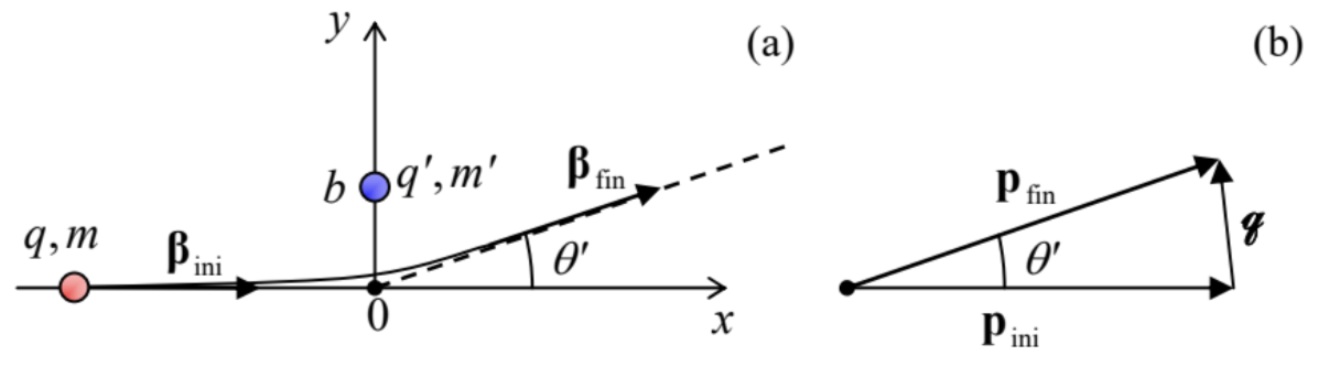Fig. 10.13. The basic geometry of the bremsstrahlung and the Coulomb loss problems in (a) direct and (b) reciprocal spaces.

To calculate the frequency spectrum of radiation emitted during a single scattering event, it is convenient to use a byproduct of the last section’s analysis, namely Eq. (59) with the replacement (60):²⁹

$$\ I(\omega)=\frac{1}{4 \pi^{2} c} \frac{q^{2}}{4 \pi \varepsilon_{0}}\left|\int_{-\infty}^{+\infty}\left[\frac{d}{d t} \frac{\mathbf{n} \times(\mathbf{n} \times \boldsymbol{\beta})}{1-\boldsymbol{\beta} \cdot \mathbf{n}} \exp \left\{i \omega\left(t-\frac{\mathbf{n} \cdot \mathbf{r}^{\prime}}{c}\right)\right\}\right]_{\mathrm{ret}} d t_{\mathrm{ret}}\right|^{2}.\tag{10.75}$$

A typical duration $\ \tau$ of a single scattering event we are discussing is of the order of $\ \tau \equiv a_{0} / c \sim\left(10^{-10}\right.\mathrm{m}) /\left(3 \times 10^{8} \mathrm{~m} / \mathrm{s}\right) \sim 10^{-18}s$ in solids, and only an order of magnitude longer in gases at ambient conditions. This is why for most frequencies of interest, from zero all the way up to at least soft X-rays,³⁰ we can use the so-called low-frequency approximation, taking the exponent in Eq. (75) for 1 through the whole collision event, i.e. the integration interval. This approximation immediately yields

$$\ \text{Brems-strahlung: single collision}\quad\quad\quad\quad I(\omega)=\frac{1}{4 \pi^{2} c} \frac{q^{2}}{4 \pi \varepsilon_{0}}\left|\frac{\mathbf{n} \times\left(\mathbf{n} \times \boldsymbol{\beta}_{\mathrm{fin}}\right)}{1-\boldsymbol{\beta}_{\mathrm{fin}} \cdot \mathbf{n}}-\frac{\mathbf{n} \times\left(\mathbf{n} \times \boldsymbol{\beta}_{\mathrm{ini}}\right)}{1-\boldsymbol{\beta}_{\mathrm{ini}} \cdot \mathbf{n}}\right|^{2}.\tag{10.76}$$

In the non-relativistic limit $\ \left(\beta_{\text {ini }}, \beta_{\text {fin }}<<1\right)$, this formula is reduced to the following result:

$$\ I(\omega)=\frac{1}{4 \pi^{2} c} \frac{q^{2}}{4 \pi \varepsilon_{0}} \frac{g^{2}}{m^{2} c^{2}} \sin ^{2} \theta$$

(which may be derived from Eq. (8.27) as well), where $\ g$ is the momentum transferred from the scattering center to the scattered charge (Fig. 13b):³¹

$$\ \boldsymbol{g} \equiv \mathbf{p}_{\text {fin }}-\mathbf{p}_{\text {ini }}=m \Delta \mathbf{u}=m c \Delta \boldsymbol{\beta}=m c\left(\boldsymbol{\beta}_{\text {fin }}-\boldsymbol{\beta}_{\text {ini }}\right),\tag{10.78}$$

and $\ \theta$ (not to be confused with the particle scattering angle $\ \theta^{\prime}$ shown in Fig. 13!) is the angle between the vector $\ \mathbf{g}$ and the direction n toward the observer – at the collision moment.

The most important feature of the result (77)-(78) is the frequency-independent (“white”) spectrum of the radiation, very typical for any rapid leaps that may be approximated as delta functions of time.³² (Note, however, that Eq. (77) implies a fixed value of $\ q$, so that the statistics of this parameter, to be discussed in a minute, may “color” the radiation.)

Note also the “doughnut-shaped” angular distribution of the radiation, typical for non-relativistic systems, with the symmetry axis directed along the momentum transfer vector $\ \mathbf{g}$. In particular, this means that in typical cases when $\ \left|\theta^{\prime}\right|<<1$, i.e. $\ g<<p$, when the vector $\ \mathbf{g}$ is nearly normal to the vector $\ \mathbf{p}_{\text {ini }}$ (see, e.g., the example shown in Fig. 13b), the bremsstrahlung produces a significant radiation flow in the direction back to the particle source – the fact significant for the operation of X-ray tubes.

Now integrating Eq. (77) over all wave propagation angles, just as we did for the instant radiation power in Sec. 8.2, we get the following spectral density of the particle energy loss,

$$\ -\frac{d \mathscr{E}}{d \omega}=\oint_{4 \pi} I(\omega) d \Omega=\frac{2}{3 \pi c} \frac{q^{2}}{4 \pi^{2} \varepsilon_{0}} \frac{g^{2}}{m^{2} c^{2}}.\tag{10.79}$$

In most applications of the bremsstrahlung theory (as in most scattering problems³³), the impact parameter $\ b$ (Fig. 13a), and hence the scattering angle $\ \theta^{\prime}$ and the transferred momentum $\ \boldsymbol{g}$, have to be

considered random. For elastic $\ \left(\beta_{\text {ini }}=\beta_{\text {fin }} \equiv \beta\right)$ Coulomb collisions we can use the so-called Rutherford formula for the differential cross-section of scattering³⁴

$$\ \frac{d \sigma}{d \Omega^{\prime}}=\left(\frac{q q^{\prime}}{4 \pi \varepsilon_{0}}\right)^{2}\left(\frac{1}{2 p c \beta}\right)^{2} \frac{1}{\sin ^{4}\left(\theta^{\prime} / 2\right)}.\tag{10.80}$$

Here $\ d \sigma=2 \pi b d b$ is the elementary area of the sample cross-section (as visible from the direction of incident particles) corresponding to particle scattering into an elementary body angle³⁵

$$\ d \Omega^{\prime}=2 \pi \sin \theta^{\prime}\left|d \theta^{\prime}\right|.\tag{10.81}$$

Differentiating the geometric relation, which is evident from Fig. 13b,

$$\ \boldsymbol{g}=2 p \sin \frac{\theta^{\prime}}{2},\tag{10.82}$$

we may represent Eq. (80) in a more convenient form

$$\ \frac{d \sigma}{d g}=8 \pi\left(\frac{q q^{\prime}}{4 \pi \varepsilon_{0}}\right)^{2} \frac{1}{u^{2} g^{3}}.\tag{10.83}$$

Now combining Eqs. (79) and (83), we get

$$\ -\frac{d \mathscr{E}}{d \omega} \frac{d \sigma}{d g}=\frac{16}{3} \frac{q^{2}}{4 \pi \varepsilon_{0}}\left(\frac{q q^{\prime}}{4 \pi \varepsilon_{0} m c^{2}}\right)^{2} \frac{1}{c \beta^{2}} \frac{1}{g}.\tag{10.84}$$

This product is called the differential radiation cross-section. When integrated over all values of $\ g$ (which is equivalent to averaging over all values of the impact parameter), it gives a convenient measure of the radiation intensity. Indeed, after the multiplication by the volume density $\ n$ of independent scattering centers, such integral yields the particle’s energy loss per unit bandwidth of radiation per unit path length, $\ -d^{2} \mathscr{E} / d \omega d x$. A minor problem here is that the integral of $\ 1 / g$ formally diverges at both infinite and vanishing values of $\ g$. However, these divergences are very weak (logarithmic), and the integral converges due to virtually any reason unaccounted for in our simple analysis. The standard, though slightly approximate way to account for these effects is to write

$$\ \text{Brems-strahlung: intensity}\quad\quad\quad\quad -\frac{d^{2} \mathscr{E}}{d \omega d x} \approx \frac{16}{3} n \frac{q^{2}}{4 \pi \varepsilon_{0}}\left(\frac{q q^{\prime}}{4 \pi \varepsilon_{0} m c^{2}}\right)^{2} \frac{1}{c \beta^{2}} \ln \frac{g_{\max }}{g_{\min }},\tag{10.85}$$

and then plug, instead of $\ g_{\max }$ and $\ g_{\min }$, the scales of the most important effects limiting the range of the transferred momentum’s magnitude. At the classical-mechanics analysis, according to Eq. (82), $\ g_{\max }=2p\equiv2mu$. To estimate $\ \boldsymbol{g}_{\min }$, let us note that the very small momentum transfer takes place when the impact parameter $\ b$ is very large, and hence the effective scattering time $\ \tau \sim b / \nu$ is very long. Recalling the condition of the low-frequency approximation, we may associate $\ \boldsymbol{g}_{\mathrm{min}}$ with $\ \tau \sim 1 / \omega$ and hence with $\ b \sim u \tau \sim \nu / \omega$. Since for the small scattering angles, $\ g$ is close to the impulse $\ F \tau \sim\left(q q^{\prime} / 4 \pi \varepsilon_{0} b^{2}\right) \tau$ of the Coulomb force, we get the estimate $\ \boldsymbol{g}_{\min } \sim\left(q q^{\prime} / 4 \pi \varepsilon_{0}\right) \omega / u^{2}$, and Eq. (85) should be used with

$$\ \ln \frac{g_{\max }}{g_{\min }}=\ln \left(\frac{2 m u^{3}}{\omega} / \frac{q q^{\prime}}{4 \pi \varepsilon_{0}}\right).\quad\quad\quad\quad\text{Classical brems-strahlung}\tag{10.86}$$

This is Bohr’s formula for what is called the classical bremsstrahlung. We see that the low momentum cutoff indeed makes the spectrum slightly colored, with more energy going to lower frequencies. There is even a formal divergence at $\ \omega \rightarrow 0$; however, this divergence is integrable, so it does not present a problem for finding the total energy radiative losses $\ (-d \mathscr{E} / d x)$ as an integral of Eq. (86) over all radiated frequencies $\ \omega$. A larger problem for this procedure is the upper integration limit, $\ \omega \rightarrow \infty$, at which the integral diverges. This means that our approximate description, which considers the collision as an elastic process, becomes invalid, and needs to be amended by taking into account the difference between the initial and final kinetic energies of the particle due to radiation of the energy quantum $\ \hbar \omega$ of the emitted photon, so that

$$\ \frac{p_{\text {ini }}^{2}}{2 m}-\frac{p_{\text {fin }}^{2}}{2 m}=\hbar \omega, \quad \text { i.e. } \frac{p_{\text {ini }}^{2}}{2 m}=\mathscr{E}, \quad \frac{p_{\text {fin }}^{2}}{2 m}=\mathscr{E}-\hbar \omega,\tag{10.87}$$

As a result, taking into account that the minimum and maximum values of $\ g$ correspond to, respectively, the parallel and antiparallel alignments of the vectors $\ \mathbf{p}_{\text {ini }}$ and $\ \mathbf{p}_{\text {fin }}$, we get

$$\ \ln \frac{\boldsymbol{g}_{\max }}{\boldsymbol{g}_{\min }}=\ln \frac{p_{\text {ini }}+p_{\text {fin }}}{p_{\text {ini }}-p_{\text {fin }}} \equiv \ln \frac{\left(p_{\text {ini }}+p_{\text {fin }}\right)^{2} / 2 m}{\left(p_{\text {ini }}^{2}-p_{\text {fin }}^{2}\right) / 2 m}=\ln \frac{\left[\mathscr{E}^{1 / 2}+(\mathscr{E}-\hbar \omega)^{1 / 2}\right]^{2}}{\hbar \omega},\quad\quad\quad\quad\text{Quantum brems-strahlung}\tag{10.88}$$

Plugged into Eq. (85), this expression yields the so-called Bethe-Heitler formula for quantum bremsstrahlung.³⁶ Note that at this approach, $\ g_{\mathrm{max}}$ is close to that of the classical approximation, but $\ g_{\mathrm{min}}$ is of the order of $\ \hbar \omega / u$, so that

$$\ \frac{\left.\boldsymbol{g}_{\min }\right|_{\text {classical }}}{\left.\boldsymbol{g}_{\min }\right|_{\text {quantum }}} \sim \frac{\alpha {\mathscr{F}} \boldsymbol{\mathscr{F’}}}{\beta},\tag{10.89}$$

where $\ \mathscr{Z}$ and $\ \mathscr{Z’}$ are the particles’ charges in the units of $\ e$, and $\ \alpha$ is the dimensionless fine structure (“Sommerfeld”) constant,

$$\ \left.\alpha \equiv \frac{e^{2}}{4 \pi \varepsilon_{0} \hbar c}\right|_{\mathrm{SI}}=\left.\frac{e^{2}}{\hbar c}\right|_\mathrm{G a u s s i a n} \approx \frac{1}{137}<<1,\tag{10.90}$$

which is one of the basic notions of quantum mechanics.³⁷ Due to the smallness of the constant, the ratio (89) is below 1 for most cases of practical interest, and since the integral of (84) over $\ g$ is limited by the largest of all possible cutoffs $\ g_{\mathrm{min}}$, it is the Bethe-Heitler formula which should be used.

Now nothing prevents us from calculating the total radiative losses of energy per unit length:

$$\ -\frac{d \mathscr{E}}{d x}=\int_{0}^{\infty}\left(-\frac{d^{2} \mathscr{E}}{d \omega d z}\right) d \omega=\frac{16}{3} n \frac{q^{2}}{4 \pi \varepsilon_{0} c}\left(\frac{q q^{\prime}}{4 \pi \varepsilon_{0} m c^{2}}\right)^{2} \frac{1}{\beta^{2}} 2 \int_{0}^{\omega_{\max }} \ln \frac{\mathscr{E}^{1 / 2}-(\mathscr{E}-\hbar \omega)^{1 / 2}}{(\hbar \omega)^{1 / 2}} d \omega,\tag{10.91}$$

where $\ \hbar \omega_{\max }=\mathscr{E}$ is the maximum energy of the radiation quantum. By introducing the dimensionless integration variable $\ \xi \equiv \hbar \omega / \mathscr{E}=2 \hbar \omega /\left(m u^{2} / 2\right)$, this integral is reduced to table one,³⁸ and we get

$$\ -\frac{d \mathscr{E}}{d x}=\frac{16}{3} n \frac{q^{2}}{4 \pi \varepsilon_{0} c}\left(\frac{q q^{\prime}}{4 \pi \varepsilon_{0} m c^{2}}\right)^{2} \frac{1}{\beta^{2}} \frac{u^{2}}{\hbar} \equiv \frac{16}{3} n\left(\frac{q^{\prime 2}}{4 \pi \varepsilon_{0} \hbar c}\right)\left(\frac{q^{2}}{4 \pi \varepsilon_{0}}\right)^{2} \frac{1}{m c^{2}}.\tag{10.92}$$

In my usual style, at this point I would give you an estimate of the losses for a typical case; however, let me first discuss a parallel particle energy loss mechanism, the so called Coulomb losses, due to the transfer of mechanical impulse from the scattered particle to the scattering centers. (This energy eventually goes into an increase of the thermal energy of the scattering medium, rather than to the electromagnetic radiation.)

Using Eqs. (9.139) for the electric field of a linearly moving charge q, we can readily find the momentum it transfers to the counterpart charge $\ q’$:³⁹

$$\ \Delta p^{\prime}=\left|\left(\Delta p^{\prime}\right)_{y}\right|=\left|\int_{-\infty}^{+\infty}\left(\dot{p}^{\prime}\right)_{y} d t\right|=\left|\int_{-\infty}^{+\infty} q^{\prime} E_{y} d t\right|=\frac{q q^{\prime}}{4 \pi \varepsilon_{0}} \int_{-\infty}^{+\infty} \frac{\gamma b}{\left(b^{2}+\gamma^{2} u^{2} t^{2}\right)^{3 / 2}} d t=\frac{q q^{\prime}}{4 \pi \varepsilon_{0}} \frac{2}{b u}.\tag{10.93}$$

Hence, the kinetic energy acquired by the scattering particle (and hence to the loss of the energy $\ \mathscr{E}$ of the incident particle) is

$$\ -\Delta \mathscr{E}=\frac{\left(\Delta p^{\prime}\right)^{2}}{2 m^{\prime}}=\left(\frac{q q^{\prime}}{4 \pi \varepsilon_{0}}\right)^{2} \frac{2}{m^{\prime} u^{2} b^{2}}.\tag{10.94}$$

Such elementary energy losses have to be summed up over all collisions, with random values of the impact parameter $\ b$. At the scattering center density $\ n$, the number of collisions per small path length $\ dx$ per small range $\ db$ is $\ d N=n 2 \pi b d b d x$, so that

$$\ \text{Coulomb losses}\quad\quad\quad\quad -\frac{d \mathscr{E}}{d x}=-\int \Delta \mathscr{E}d N=n\left(\frac{q q^{\prime}}{4 \pi \varepsilon_{0}}\right)^{2} \frac{2}{m^{\prime} u^{2}} 2 \pi \int_{b_{\min }}^{b_{\max }} \frac{d b}{b}=4 \pi n\left(\frac{q q^{\prime}}{4 \pi \varepsilon_{0}}\right)^{2} \frac{\ln B}{m^{\prime} u^{2}}, \quad \text { where } B \equiv \frac{b_{\max }}{b_{\min }}.\tag{10.95}$$

Here, at the last step, the logarithmic integral over $\ b$ was treated similarly to that over $\ g$ in the bremsstrahlung theory. This approximation is adequate because the ratio $\ b_{\max } / b_{\min }$ is much larger than 1. Indeed, $\ b_{\min }$ may be estimated from $\ \left(\Delta p^{\prime}\right)_{\max } \sim p=\gamma m u$. For this value, Eq. (93) with $\ q^{\prime} \sim q$ gives $\ b_{\min } \sim r_c$ (see Eq. (8.41) and its discussion), which, for elementary particles, is of the order of $\ 10^{-15} \mathrm{~m}$. On the other hand, for the most important case when the Coulomb energy absorbers are electrons (which, according to Eq. (94), are the most efficient ones, due to their very low mass $\ m^{\prime}$), $\ b_{\max }$ may be estimated from the condition $\ \tau=b / \gamma u \sim 1 / \omega_{\min }$, where $\ \omega_{\min } \sim 10^{16} \mathrm{~s}^{-1}$ is the characteristic frequency of electron transitions in atoms. (Quantum mechanics forbids such energy transfer at lower frequencies.) From here, we have estimate $\ b_{\max } \sim \gamma u / \omega_{\min }$, so that

$$\ B \equiv \frac{b_{\max }}{b_{\min }} \sim \frac{\gamma u}{r_{\mathrm{c}} \omega_{\min }},\tag{10.96}$$

for $\ \gamma \sim 1$ and $\ u \sim c \approx 3 \times 10^{8} \mathrm{~m} / \mathrm{s}$ giving $\ b_{\max } \sim 3 \times 10^{-8} \mathrm{~m}$, so that $\ B \sim 10^{9}$ (give or take a couple of orders of magnitude – this does not change the estimate $\ \ln B \approx 20$ too much).⁴⁰

Now we can compare the non-radiative Coulomb losses (95) with the radiative losses due to the bremsstrahlung, given by Eq. (92):

$$\ \frac{-\left.d \mathscr{E}\right|_{\text {radiation }}}{-\left.d \mathscr{E}\right|_{\text {Coulomb }}} \sim \alpha \mathscr{F}{\mathscr{F’}} \frac{m^{\prime}}{m} \beta^{2} \frac{1}{\ln B},\tag{10.97}$$

Since $\ \alpha \sim 10^{-2}<<1$, for non-relativistic particles $\ (\beta<<1)$ the bremsstrahlung losses of energy are much lower (this is why I did not want to rush with their estimates), and only for ultra-relativistic particles, the relation may be opposite.

According to Eqs. (95)-(96), for electron-electron scattering $\ \left(q=q^{\prime}=-e, m=m^{\prime}=m_{\mathrm{e}}\right)$,⁴¹ at the value $\ n=6 \times 10^{26} \mathrm{~m}^{-3}$ typical for air at ambient conditions, the characteristic length of energy loss,

$$\ l_{\mathrm{c}} \equiv \frac{\mathscr{E}}{\left(-d\mathscr{E} / d x\right)},\tag{10.98}$$

for electrons with kinetic energy $\ \mathscr{E}=6 \mathrm{keV}$ is close to $\ 2 \times 10^{-4} \mathrm{~m} \equiv 0.2 \mathrm{~mm}$. (This is why we need high
vacuum in particle accelerators and electron microscope columns!) Since $\ l_{\mathrm{c}} \propto \mathscr{E}^{2}$, more energetic particles penetrate to matter deeper, until the bremsstrahlung steps in, and limits this trend at very high energies.

---

Reference

²⁸ Such X-ray radiation had been first observed experimentally, though not correctly interpreted by N. Tesla in 1887, i.e. before it was rediscovered and studied in detail by W. Röntgen.

²⁹ In publications on this topic (whose development peak was in the 1920s-1930s), the Gaussian units are more common, and the uppercase letter $\ Z$ is usually reserved for expressing charges as multiples the fundamental charge $\ e$, rather than for the wave impedance. This is why, in order to avoid confusion and facilitate the comparison with other texts, in this section I (still staying with the SI units used throughout my series) will use the fraction $\ 1 / \varepsilon_{0} c$, instead of its equivalent $\ Z_{0}$, for the free-space wave impedance, and write the coefficients in a form that makes the transfer to the Gaussian units elementary: it is sufficient to replace all $\ \left(q q^{\prime} / 4 \pi \varepsilon_{0}\right)_{\mathrm{SI}}$ with $\ \left(q q^{\prime}\right)_{\text {Gaussian }}$. In the (rare) cases when I spell out the charge values, I will use a different font: $\ q \equiv \mathscr{F} e, q^{\prime} \equiv \mathscr{F}^{\prime} e$.

³⁰ A more careful analysis shows that this approximation is actually quite reasonable up to much higher frequencies, of the order of $\ \gamma^{2} / \tau$.

³¹ Please note the font-marked difference between this variable $\ (\boldsymbol{g})$ and the particle’s electric charge $\ (q)$.

³² This is the basis, in particular, of the so-called High-Harmonic Generation (HHG) effect, discovered in 1977, which takes place at the irradiation of gases by intensive laser beams. The high electric field of the beam strips valent electrons from initially neutral atoms, and accelerates them away from the remaining ions, just to slam them back into the ions as the field’s polarity changes in time. The electrons change their momentum sharply during their recombination with the ions, resulting in bremsstrahlung-like radiation. The spectrum of radiation from each such event obeys Eq. (77), but since the ionization/acceleration/recombination cycles repeat periodically with the frequency $\ \omega_{0}$ of the laser field, the final spectrum consists of many equidistant lines, with frequencies $\ n \omega_{0}$. The classical theory of the bremsstrahlung does not give a cutoff $\ \omega_{\max }=n_{\max } \omega_{0}$ of the spectrum; this limit is imposed by quantum mechanics: $\ \hbar \omega_{\max } \sim \mathscr{E}_{\mathrm{p}}$, where the so-called ponderomotive energy $\ \mathscr{E}_{\mathrm{p}}=\left(e E_{0} / \omega_{0}\right)^{2} / 4 m_{\mathrm{e}}$ is the average kinetic energy given to a free electron by the periodic electric field of the laser beam, with amplitude $\ E_{0}$. In practice, $\ n_{\max }$ may be as high as ~100, enabling alternative compact sources of X-ray radiation. For a detailed quantitative theory of this effect, see, for example, M. Lewenstein et al., Phys. Rev. A 49, 2117 (1994).

³³ See, e.g., CM Sec. 3.5 and QM Sec. 3.3.

³⁴ See, e.g., CM Eq. (3.73) with $\ \alpha=q q^{\prime} / 4 \pi \varepsilon_{0}$. In the form used in Eq. (80), the Rutherford formula is also valid for small-angle scattering of relativistic particles, the criterion being $\ |\Delta \boldsymbol{\beta}|<<2 / \gamma$.

³⁵ Again, the angle $\ \theta’$ and the differential $\ d\Omega’$, describing the scattered particles (see Fig.13) should not be confused with the parameters $\ \theta$ and $\ d\Omega$ describing the radiation emitted at the scattering event.

³⁶ The modifications of this formula necessary for the relativistic description are surprisingly minor – see, e.g., Chapter 15 in J. Jackson, Classical Electrodynamics, 3^rd ed., Wiley 1999. For even more detail, the standard reference monograph on bremsstrahlung is W. Heitler, The Quantum Theory of Radiation, 3^rd ed., Oxford U. Press 1954 (reprinted in 1984 and 2010 by Dover).

³⁷ See, e.g., QM Secs. 4.4, 6.3, 6.4, 9.3, 9.5, and 9.7.

³⁸ See, e.g., MA Eq. (6.14).

³⁹ According to Eq. (9.139), $\ E_{z}=0$, while the net impulse of the longitudinal force $\ q^{\prime} E_{x}$ is zero, so that Eq. (93) gives the full momentum transfer.

⁴⁰ A quantum analysis (carried out by Hans Bethe in 1940) replaces, in Eq. (95), $\ \ln B$ with $\ \ln \left(2 \gamma^{2} m u^{2} / \hbar\langle\omega\rangle\right)-\beta^{2}$, where $\ \langle\omega\rangle$ is the average frequency of the atomic quantum transitions weight by their oscillator strength. This refinement does not change the estimate given below. Note that both the classical and quantum formulas describe a fast increase (as $\ 1 / \beta$) of the energy loss rate $\ (-d \mathscr{E} / d x)$ at $\ \gamma \rightarrow 1$, and its slow increase (as $\ \ln \gamma$) at $\ \gamma \rightarrow \infty$, so that the losses have a minimum at $\ (\gamma-1) \sim 1$.

⁴¹ Actually, the above analysis has neglected the change of momentum of the incident particle. This is legitimate at $\ m^{\prime}<<m$, but for $\ m=m^{\prime}$ the change approximately doubles the energy losses. Still, this does not change the order of magnitude of the estimate.