
1.5: 1.5 Trigonometric Functions


- Last updated
- Apr 30, 2021
- Save as PDF

\newcommand{\vecs}[1]{\overset { \scriptstyle \rightharpoonup} {\mathbf{#1}} }
\newcommand{\vecd}[1]{\overset{-\!-\!\rightharpoonup}{\vphantom{a}\smash {#1}}}
\newcommand{\id}{\mathrm{id}} \newcommand{\Span}{\mathrm{span}}
( \newcommand{\kernel}{\mathrm{null}\,}\) \newcommand{\range}{\mathrm{range}\,}
\newcommand{\RealPart}{\mathrm{Re}} \newcommand{\ImaginaryPart}{\mathrm{Im}}
\newcommand{\Argument}{\mathrm{Arg}} \newcommand{\norm}[1]{\| #1 \|}
\newcommand{\inner}[2]{\langle #1, #2 \rangle}
\newcommand{\Span}{\mathrm{span}}
\newcommand{\id}{\mathrm{id}}
\newcommand{\Span}{\mathrm{span}}
\newcommand{\kernel}{\mathrm{null}\,}
\newcommand{\range}{\mathrm{range}\,}
\newcommand{\RealPart}{\mathrm{Re}}
\newcommand{\ImaginaryPart}{\mathrm{Im}}
\newcommand{\Argument}{\mathrm{Arg}}
\newcommand{\norm}[1]{\| #1 \|}
\newcommand{\inner}[2]{\langle #1, #2 \rangle}
\newcommand{\Span}{\mathrm{span}} \newcommand{\AA}{\unicode[.8,0]{x212B}}
\newcommand{\vectorA}[1]{\vec{#1}} % arrow
\newcommand{\vectorAt}[1]{\vec{\text{#1}}} % arrow
\newcommand{\vectorB}[1]{\overset { \scriptstyle \rightharpoonup} {\mathbf{#1}} }
\newcommand{\vectorC}[1]{\textbf{#1}}
\newcommand{\vectorD}[1]{\overrightarrow{#1}}
\newcommand{\vectorDt}[1]{\overrightarrow{\text{#1}}}
\newcommand{\vectE}[1]{\overset{-\!-\!\rightharpoonup}{\vphantom{a}\smash{\mathbf {#1}}}}
\newcommand{\vecs}[1]{\overset { \scriptstyle \rightharpoonup} {\mathbf{#1}} }
\newcommand{\vecd}[1]{\overset{-\!-\!\rightharpoonup}{\vphantom{a}\smash {#1}}}
\newcommand{\avec}{\mathbf a} \newcommand{\bvec}{\mathbf b} \newcommand{\cvec}{\mathbf c} \newcommand{\dvec}{\mathbf d} \newcommand{\dtil}{\widetilde{\mathbf d}} \newcommand{\evec}{\mathbf e} \newcommand{\fvec}{\mathbf f} \newcommand{\nvec}{\mathbf n} \newcommand{\pvec}{\mathbf p} \newcommand{\qvec}{\mathbf q} \newcommand{\svec}{\mathbf s} \newcommand{\tvec}{\mathbf t} \newcommand{\uvec}{\mathbf u} \newcommand{\vvec}{\mathbf v} \newcommand{\wvec}{\mathbf w} \newcommand{\xvec}{\mathbf x} \newcommand{\yvec}{\mathbf y} \newcommand{\zvec}{\mathbf z} \newcommand{\rvec}{\mathbf r} \newcommand{\mvec}{\mathbf m} \newcommand{\zerovec}{\mathbf 0} \newcommand{\onevec}{\mathbf 1} \newcommand{\real}{\mathbb R} \newcommand{\twovec}[2]{\left[\begin{array}{r}#1 \\ #2 \end{array}\right]} \newcommand{\ctwovec}[2]{\left[\begin{array}{c}#1 \\ #2 \end{array}\right]} \newcommand{\threevec}[3]{\left[\begin{array}{r}#1 \\ #2 \\ #3 \end{array}\right]} \newcommand{\cthreevec}[3]{\left[\begin{array}{c}#1 \\ #2 \\ #3 \end{array}\right]} \newcommand{\fourvec}[4]{\left[\begin{array}{r}#1 \\ #2 \\ #3 \\ #4 \end{array}\right]} \newcommand{\cfourvec}[4]{\left[\begin{array}{c}#1 \\ #2 \\ #3 \\ #4 \end{array}\right]} \newcommand{\fivevec}[5]{\left[\begin{array}{r}#1 \\ #2 \\ #3 \\ #4 \\ #5 \\ \end{array}\right]} \newcommand{\cfivevec}[5]{\left[\begin{array}{c}#1 \\ #2 \\ #3 \\ #4 \\ #5 \\ \end{array}\right]} \newcommand{\mattwo}[4]{\left[\begin{array}{rr}#1 \amp #2 \\ #3 \amp #4 \\ \end{array}\right]} \newcommand{\laspan}[1]{\text{Span}\{#1\}} \newcommand{\bcal}{\cal B} \newcommand{\ccal}{\cal C} \newcommand{\scal}{\cal S} \newcommand{\wcal}{\cal W} \newcommand{\ecal}{\cal E} \newcommand{\coords}[2]{\left\{#1\right\}_{#2}} \newcommand{\gray}[1]{\color{gray}{#1}} \newcommand{\lgray}[1]{\color{lightgray}{#1}} \newcommand{\rank}{\operatorname{rank}} \newcommand{\row}{\text{Row}} \newcommand{\col}{\text{Col}} \renewcommand{\row}{\text{Row}} \newcommand{\nul}{\text{Nul}} \newcommand{\var}{\text{Var}} \newcommand{\corr}{\text{corr}} \newcommand{\len}[1]{\left|#1\right|} \newcommand{\bbar}{\overline{\bvec}} \newcommand{\bhat}{\widehat{\bvec}} \newcommand{\bperp}{\bvec^\perp} \newcommand{\xhat}{\widehat{\xvec}} \newcommand{\vhat}{\widehat{\vvec}} \newcommand{\uhat}{\widehat{\uvec}} \newcommand{\what}{\widehat{\wvec}} \newcommand{\Sighat}{\widehat{\Sigma}} \newcommand{\lt}{<} \newcommand{\gt}{>} \newcommand{\amp}{&} \definecolor{fillinmathshade}{gray}{0.9}Another extremely important group of functions are the fundamental trignonometric functions \sin, \cos, and \tan. These can be defined in terms of the geometric ratios of the sides of right-angled triangles, as shown below:
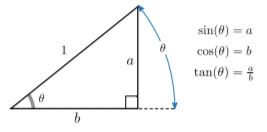
If we use this basic definition, the domain is \theta \in [0, \,\pi/2), where the input angle \theta is given in radians.
We can generalize the definition using the following scheme, which allows for negative values of a and/or b:
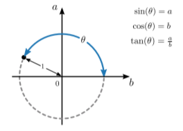
With this, the domain is extended to \theta \in [0,\,2\pi). We can further extend the domain to all real numbers, \theta \in \mathbb{R}, by treating input values modulo 2\pi as equivalent; in other words, f(\theta + 2\pi) = f(\theta). With this generalization, the trigonometric functions become many-to-one functions.
According to the Pythagorean theorem, \big[\sin(\theta)\big]^2 + \big[\cos(\theta)\big]^2 = 1. Using this, we can go on to prove a variety of identities, like the addition identities \begin{align} \sin(\theta_1 + \theta_2) &= \sin(\theta_1) \cos(\theta_2) + \cos(\theta_1)\sin(\theta_2) \\ \cos(\theta_1 + \theta_2) &= \cos(\theta_1) \cos(\theta_2) - \sin(\theta_1)\sin(\theta_2)\end{align} As you may recall, the trigonometric proofs for these identities involve drawing complicated triangle diagrams, cleverly applying the Pythagorean formula, etc. There are two problems with such proofs: (i) they require some ingenuity in the construction of the triangle diagrams, and (ii) it may not be obvious whether the proofs work if the angles lie outside [0,\pi/2).
Happily, there is a solution to both problems. As we’ll soon see, such trigonometric identities can be proven algebraically by using complex numbers.