5.6: Longitudinally and Transversely Separated Points

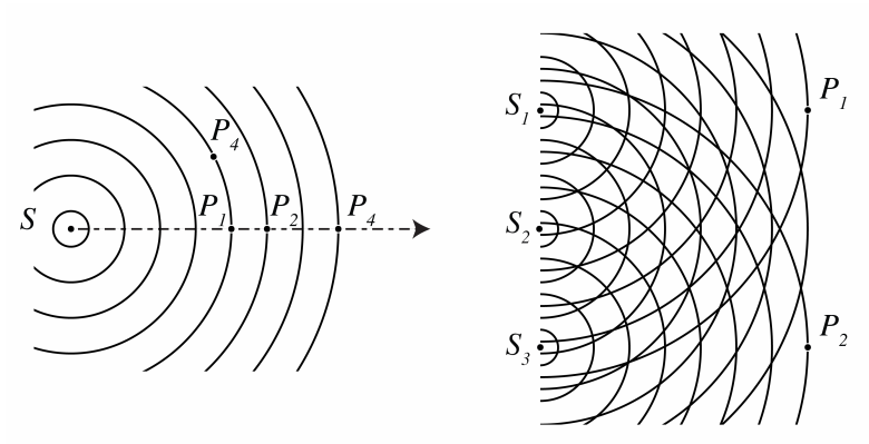
Consider two points that are separated along the mean direction of propagation of the light (imagine that the two points are situated along the same ray). If the phase is known in one of these points at a certain instant, then we can predict the phase in the other point at the same instant of time, provided that the distance between the points is less than the coherence length \(\Delta \ell_{c}\). We call points separated parallel to the mean direction of propagation of the light longitudinally separated points. In Figure \(\PageIndex{1}\) at the left, the spherical wave fronts of a purely monochromatic point source are shown. The field is fully coherent. What happens in point \(P_{1}\) will some time later happen in \(P_{2}\) and still a bit later in \(P_{3}\) etc. However, if the point source is not monochromatic, and the phase of the field changes randomly from time to time as in Figure 5.3.1, there is hardly any correlation of the wave at points that are longitudinally far apart such as \(P_{1}\) and \(P_{3}\). Nevertheless, the waves are not totally unpredictable: the behaviour at points closer together such as \(P_{1}\) and \(P_{2}\) are still somewhat correlated. When the distance between longitudinally separated points is larger than the coherence length \(\Delta \ell_{c}\), the mutual coherence between these points is negligible. Michelson’s interferometer is ideally suited to determine the coherence time and coherence length and therefore also the mutual coherence of longitudinally separated points. Because the distance between longitudinally separated points is equal to the difference in the distances between the source and each of points, we can alternatively say that two longitudinally separated points are coherent if the difference in distances from the source to these points is smaller than the coherence length.

Next consider points which are separated in a direction perpendicular to the mean direction of propagation of the light. Such points are called transversely separated. The mutual coherence of the fields at these points for zero (or small) time delay is called spatial coherence. Note that, even when the source is not monochromatic and the coherence time of the source is short, the fields in the transversely separated points \(P_{1}\) and \(P_{4}\) at the left of Figs. \(\PageIndex{1}\) are always completely correlated because they are on the same wavefront. In fact, the distances between the source and these points identical.

The situation is different when the source is not a single point source but consists of several mutually completely incoherent point sources as at the right of Figure Figs. \(\PageIndex{1}\). First of all, the fields from different point sources can not interfere with each other because, during the integration time of a typical detector, fields of different point sources undergo thousands of random uncorrelated phase jumps. Furthermore, the difference between the distances of two points such as \(P_{1}\) and \(P_{2}\) at the right of Figure Figs. \(\PageIndex{1}\), cannot be zero for all point sources. Hence, the contributions of the individual point sources to the total fields in the two points can not all be in phase or out of phase together. Stated differently, transversely separated points that are on the same wavefront emitted by a particular point source are coherent, but these points cannot be on the same wave fronts for all point sources. However, when the differences of distances from the transversely separated points \(P_{1}\) and \(P_{2}\) at the right of Figure Figs. \(\PageIndex{1}\) to each of the point sources are smaller than the coherence length \(\Delta \ell_{c}\), the fields at the same instant (zero time delay) at the transversely separated points are nevertheless coherent.

The spatial coherence can be experimentally investigated by putting an opaque mask orthogonal to the mean direction of propagation of the light, with two small holes at the points of interest. The fields transmitted by the holes are made to interfere at a screen at a large distance, as shown in Figure 5.6.1. This is the famous Young experiment. The field due to one point source in the two holes can interfere on the screen, but contributions from different point sources cannot. Hence the fringe pattern is the sum of the intensity patterns due to the individual point sources and the contrast in the fringe pattern of this total intensity pattern is a measure of the degree of spatial coherence of the disturbances at the two transversely separated points (holes).

We conclude that for both longitudinally and transversely separated points, and in fact more generally for any pair of points,

The fields in two points considered at the same instant (no time delay) are coherent when the differences in distances between these points and any of the point sources in the extended source are smaller than the coherence length \(\Delta \ell_{c}\).

This result will be derived more rigorously in Section \(5.7\).

Figure \(\PageIndex{1}\): Left: the waves emitted by a single monochromatic point sources are perfectly (temporally and spatially) coherent. If the point source is not monochromatic, the fields at points that are longitudinally separated such as \(P_{1}, P_{2}\) and \(P_{3}\) are more coherent the smaller the difference in distance is of these points to the source. Transversely separated points such as \(P_{1}, P_{4}\) in the left figure, are fully coherent because they are on the same wave front. When there are more point sources such as in the right figure, the degree of spatial coherence of transversally separated points such as \(P_{1}\) and \(P_{2}\), depends on the differences in distance of each point source to the points \(P_{1}, P_{2}\).