7.3: Amplification
- Page ID
- 57635
\( \newcommand{\vecs}[1]{\overset { \scriptstyle \rightharpoonup} {\mathbf{#1}} } \)
\( \newcommand{\vecd}[1]{\overset{-\!-\!\rightharpoonup}{\vphantom{a}\smash {#1}}} \)
\( \newcommand{\dsum}{\displaystyle\sum\limits} \)
\( \newcommand{\dint}{\displaystyle\int\limits} \)
\( \newcommand{\dlim}{\displaystyle\lim\limits} \)
\( \newcommand{\id}{\mathrm{id}}\) \( \newcommand{\Span}{\mathrm{span}}\)
( \newcommand{\kernel}{\mathrm{null}\,}\) \( \newcommand{\range}{\mathrm{range}\,}\)
\( \newcommand{\RealPart}{\mathrm{Re}}\) \( \newcommand{\ImaginaryPart}{\mathrm{Im}}\)
\( \newcommand{\Argument}{\mathrm{Arg}}\) \( \newcommand{\norm}[1]{\| #1 \|}\)
\( \newcommand{\inner}[2]{\langle #1, #2 \rangle}\)
\( \newcommand{\Span}{\mathrm{span}}\)
\( \newcommand{\id}{\mathrm{id}}\)
\( \newcommand{\Span}{\mathrm{span}}\)
\( \newcommand{\kernel}{\mathrm{null}\,}\)
\( \newcommand{\range}{\mathrm{range}\,}\)
\( \newcommand{\RealPart}{\mathrm{Re}}\)
\( \newcommand{\ImaginaryPart}{\mathrm{Im}}\)
\( \newcommand{\Argument}{\mathrm{Arg}}\)
\( \newcommand{\norm}[1]{\| #1 \|}\)
\( \newcommand{\inner}[2]{\langle #1, #2 \rangle}\)
\( \newcommand{\Span}{\mathrm{span}}\) \( \newcommand{\AA}{\unicode[.8,0]{x212B}}\)
\( \newcommand{\vectorA}[1]{\vec{#1}} % arrow\)
\( \newcommand{\vectorAt}[1]{\vec{\text{#1}}} % arrow\)
\( \newcommand{\vectorB}[1]{\overset { \scriptstyle \rightharpoonup} {\mathbf{#1}} } \)
\( \newcommand{\vectorC}[1]{\textbf{#1}} \)
\( \newcommand{\vectorD}[1]{\overrightarrow{#1}} \)
\( \newcommand{\vectorDt}[1]{\overrightarrow{\text{#1}}} \)
\( \newcommand{\vectE}[1]{\overset{-\!-\!\rightharpoonup}{\vphantom{a}\smash{\mathbf {#1}}}} \)
\( \newcommand{\vecs}[1]{\overset { \scriptstyle \rightharpoonup} {\mathbf{#1}} } \)
\(\newcommand{\longvect}{\overrightarrow}\)
\( \newcommand{\vecd}[1]{\overset{-\!-\!\rightharpoonup}{\vphantom{a}\smash {#1}}} \)
\(\newcommand{\avec}{\mathbf a}\) \(\newcommand{\bvec}{\mathbf b}\) \(\newcommand{\cvec}{\mathbf c}\) \(\newcommand{\dvec}{\mathbf d}\) \(\newcommand{\dtil}{\widetilde{\mathbf d}}\) \(\newcommand{\evec}{\mathbf e}\) \(\newcommand{\fvec}{\mathbf f}\) \(\newcommand{\nvec}{\mathbf n}\) \(\newcommand{\pvec}{\mathbf p}\) \(\newcommand{\qvec}{\mathbf q}\) \(\newcommand{\svec}{\mathbf s}\) \(\newcommand{\tvec}{\mathbf t}\) \(\newcommand{\uvec}{\mathbf u}\) \(\newcommand{\vvec}{\mathbf v}\) \(\newcommand{\wvec}{\mathbf w}\) \(\newcommand{\xvec}{\mathbf x}\) \(\newcommand{\yvec}{\mathbf y}\) \(\newcommand{\zvec}{\mathbf z}\) \(\newcommand{\rvec}{\mathbf r}\) \(\newcommand{\mvec}{\mathbf m}\) \(\newcommand{\zerovec}{\mathbf 0}\) \(\newcommand{\onevec}{\mathbf 1}\) \(\newcommand{\real}{\mathbb R}\) \(\newcommand{\twovec}[2]{\left[\begin{array}{r}#1 \\ #2 \end{array}\right]}\) \(\newcommand{\ctwovec}[2]{\left[\begin{array}{c}#1 \\ #2 \end{array}\right]}\) \(\newcommand{\threevec}[3]{\left[\begin{array}{r}#1 \\ #2 \\ #3 \end{array}\right]}\) \(\newcommand{\cthreevec}[3]{\left[\begin{array}{c}#1 \\ #2 \\ #3 \end{array}\right]}\) \(\newcommand{\fourvec}[4]{\left[\begin{array}{r}#1 \\ #2 \\ #3 \\ #4 \end{array}\right]}\) \(\newcommand{\cfourvec}[4]{\left[\begin{array}{c}#1 \\ #2 \\ #3 \\ #4 \end{array}\right]}\) \(\newcommand{\fivevec}[5]{\left[\begin{array}{r}#1 \\ #2 \\ #3 \\ #4 \\ #5 \\ \end{array}\right]}\) \(\newcommand{\cfivevec}[5]{\left[\begin{array}{c}#1 \\ #2 \\ #3 \\ #4 \\ #5 \\ \end{array}\right]}\) \(\newcommand{\mattwo}[4]{\left[\begin{array}{rr}#1 \amp #2 \\ #3 \amp #4 \\ \end{array}\right]}\) \(\newcommand{\laspan}[1]{\text{Span}\{#1\}}\) \(\newcommand{\bcal}{\cal B}\) \(\newcommand{\ccal}{\cal C}\) \(\newcommand{\scal}{\cal S}\) \(\newcommand{\wcal}{\cal W}\) \(\newcommand{\ecal}{\cal E}\) \(\newcommand{\coords}[2]{\left\{#1\right\}_{#2}}\) \(\newcommand{\gray}[1]{\color{gray}{#1}}\) \(\newcommand{\lgray}[1]{\color{lightgray}{#1}}\) \(\newcommand{\rank}{\operatorname{rank}}\) \(\newcommand{\row}{\text{Row}}\) \(\newcommand{\col}{\text{Col}}\) \(\renewcommand{\row}{\text{Row}}\) \(\newcommand{\nul}{\text{Nul}}\) \(\newcommand{\var}{\text{Var}}\) \(\newcommand{\corr}{\text{corr}}\) \(\newcommand{\len}[1]{\left|#1\right|}\) \(\newcommand{\bbar}{\overline{\bvec}}\) \(\newcommand{\bhat}{\widehat{\bvec}}\) \(\newcommand{\bperp}{\bvec^\perp}\) \(\newcommand{\xhat}{\widehat{\xvec}}\) \(\newcommand{\vhat}{\widehat{\vvec}}\) \(\newcommand{\uhat}{\widehat{\uvec}}\) \(\newcommand{\what}{\widehat{\wvec}}\) \(\newcommand{\Sighat}{\widehat{\Sigma}}\) \(\newcommand{\lt}{<}\) \(\newcommand{\gt}{>}\) \(\newcommand{\amp}{&}\) \(\definecolor{fillinmathshade}{gray}{0.9}\)Amplification can be achieved by a medium with atomic resonances that are at or close to one of the resonances of the resonator. We first recall the simple theory developed by Einstein in 1916 of the dynamic equilibrium of a material in the presence of electromagnetic radiation.
7.3.1 The Einstein Coefficients
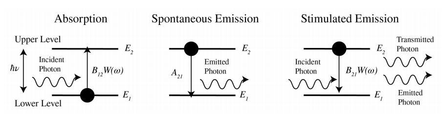
We consider two atomic energy levels \(E_{2}>E_{1}\). By absorbing a photon of energy \[\hbar \omega=E_{2}-E_{1}, \nonumber \] an atom that is initially in the lower energy state 1 can be excited to state 2 . Here \(\hbar\) is Planck’s constant: \[\hbar=\frac{6.626070040}{2 \pi} \times 10^{-34} \quad \text { Js } . \nonumber \]
Suppose \(W(\omega)\) is the time-averaged electromagnetic energy density per unit of frequency interval around frequency \(\omega\). Hence \(W\) has dimension Jsm \(^{3}\). Let \(N_{1}\) and \(N_{2}\) be the number of atoms in state 1 and 2, respectively, where \[N_{1}+N_{2}=N, \nonumber \] is the total number of atoms (which is constant). The rate of absorption is the rate of decrease of \(N_{1}\) and is proportional to the energy density and the number of atoms in state 1: \[\frac{d N_{1}}{d t}=-B_{12} N_{1} W(\omega), \quad \text { absorption, } \nonumber \] where the constant \(B_{12}>0\) has dimension \(\mathrm{m}^{3} \mathrm{~J}^{-1} \mathrm{~s}^{-2}\). Without any external influence, an atom that is in the excited state will usually transfer to state 1 within \(1 \mathrm{~ns}\) or so, while emitting a photon of energy (7.10). This process is called spontaneous emission, since it happens also without an electromagnetic field present. The rate of spontaneous emission is given by: \[\frac{d N_{2}}{d t}=-A_{21} N_{2}, \quad \text { spontaneous emission, } \nonumber \] where \(A_{21}\) has dimension \(\mathrm{s}^{-1}\). The lifetime of spontaneous transmission is \(\tau_{s p}=1 / A_{21}\). It is important to note that the spontaneously emitted photon is emitted in a random direction. Furthermore, since the radiation occurs at a random time, there is no phase relation between the spontaneously emitted field and the field that excites the atom.
It is less obvious that in the presence of an electromagnetic field of frequency close to the atomic resonance, an atom in the excited state can also be stimulated by that field to emit a photon and transfer to the lower energy state. The rate of stimulated emission is proportional to the number of excited atoms and to the energy density of the field: \[\frac{d N_{2}}{d t}=-B_{21} N_{2} W(\omega), \quad \text { stimulated emission, } \nonumber \] where \(B_{21}\) has the same dimension as \(B_{12}\). It is very important to remark that stimulated emission occurs in the same electromagnetic mode (e.g. a plane wave) as the mode of the field that excites the transmission and that the phase of the radiated field is identical to that of the exciting field. This implies that stimulated emission enhances the electromagnetic field by constructive interference. This property is crucial for the operation of the laser.
7.3.2 Relation Between the Einstein Coefficients
Relations exist between the Einstein coefficients \(A_{21}, B_{12}\) and \(B_{21}\). Consider a black body, such as a closed empty box. After a certain time, thermal equilibrium will be reached. Because there is no radiation entering the box from the outside nor leaving the box to the outside, the electromagnetic energy density is the thermal density \(W_{T}(\omega)\), which, according to Planck’s Law, is independent of the material of which the box is made and is given by: \[W_{T}(\omega)=\frac{\hbar \omega^{3}}{\pi^{2} c^{3}} \frac{1}{\exp \left(\frac{\hbar \omega}{k_{B} T}\right)-1}, \nonumber \] where \(k_{B}\) is Boltzmann’s constant: \[k_{B}=1.38064852 \times 10^{-23} \mathrm{~m}^{2} \mathrm{kgs}^{-2} \mathrm{~K}^{-1} . \nonumber \]
The rate of upward and downwards transition of the atoms in the wall of the box must be identical: \[B_{12} N_{1} W_{T}(\omega)=A_{21} N_{2}+B_{21} N_{2} W_{T}(\omega) . \nonumber \]
Hence, \[W_{T}(\omega)=\frac{A_{21}}{B_{12} N_{1} / N_{2}-B_{21}} . \nonumber \]
But in thermal equilibrium: \[\frac{N_{2}}{N_{1}}=\exp \left(-\frac{E_{2}-E_{1}}{k_{B} T}\right)=\exp \left(-\frac{\hbar \omega}{k_{B} T}\right) . \nonumber \]
By substituting (\(\PageIndex{11}\)) into (\(\PageIndex{10}\)), and comparing the result with (\(\PageIndex{7}\)), it follows that both expressions for \(W_{T}(\omega)\) are identical for all temperatures only if \[B_{12}=B_{21}, \quad A_{21}=\frac{\hbar \omega^{3}}{\pi^{2} c^{3}} B_{21} . \nonumber \]
Example For green light of \(\lambda=550 \mathrm{~nm}\), we have \(\omega / c=2 \pi / \lambda=2.8560 \times 10^{6} \mathrm{~m}^{-1}\) and thus \[\frac{A_{21}}{B_{21}}=1.5640 \times 10^{-15} \mathrm{~J} \mathrm{~s} \mathrm{~m}^{-3} . \nonumber \]
Hence the spontaneous and stimulated emission rates are equal if \(W(\omega)=1.5640 \times 10^{-15} \mathrm{Js} \mathrm{m}^{-3}\)
For a (narrow) frequency band \(\mathrm{d} \omega\) the time-averaged energy density is \(W(\omega) \mathrm{d} \omega\) and for a plane wave the energy density is related to the intensity \(I\) (i.e. the length of the time-averaged Poynting vector) as: \[W(\omega) \mathrm{d} \omega=I / c . \nonumber \]
| \(I\left(\mathrm{~W} \mathrm{~m}^{-2}\right)\) | |
|---|---|
| Mercury lamp | \(10^{4}\) |
| Continuous laser | \(10^{5}\) |
| Pulsed laser | \(10^{13}\) |
A typical value for the frequency width of a narrow emission line of an ordinary light source is: \(10^{10} \mathrm{~Hz}\), i.e. \(\mathrm{d} \omega=2 \pi \times 10^{10} \mathrm{~Hz}\). Hence, the spontaneous and stimulated emission rates are identical if the intensity is \(I=2.95 \times 10^{4} \mathrm{~W} / \mathrm{m}^{2}\). As seen from Table 7.1, only for laser light stimulated emission is larger than spontaneous emission. For classical light sources the spontaneous emission rate is much larger than the stimulated emission rate. If a beam with frequency width \(\mathrm{d} \omega\) and energy density \(W(\omega)\) d \(\omega\) propagates through a material, the rate of loss of energy is proportional to: \[\left(N_{1}-N_{2}\right) B_{12} W(\omega) . \nonumber \]
According to ( \(\PageIndex{9}\)) this is equal to the spontaneous emission rate. Indeed, the spontaneously emitted light corresponds to a loss of intensity of the beam, because it is emitted in random directions and with random phase.
When \(N_{2}>N_{1}\), the light is amplified. This state is called population inversion and it is essential for the operation of the laser. Note that the ratio of the spontaneous and stimulated emission rates is, according to (\(\PageIndex{12}\)), proportional to \(\omega^{3}\). Hence for shorter wavelengths such as \(\mathrm{x}\)-rays, it is much more difficult to make lasers than for visible light.
7.3.3 Population Inversion
For electromagnetic energy density \(W(\omega)\) per unit of frequency interval, the rate equations are \[\begin{aligned} \frac{d N_{2}}{d t} &=-A_{21} N_{2}+\left(N_{1}-N_{2}\right) B_{12} W(\omega) \\ \frac{d N_{1}}{d t} &=A_{21} N_{2}-\left(N_{1}-N_{2}\right) B_{12} W(\omega) \end{aligned} \nonumber \]
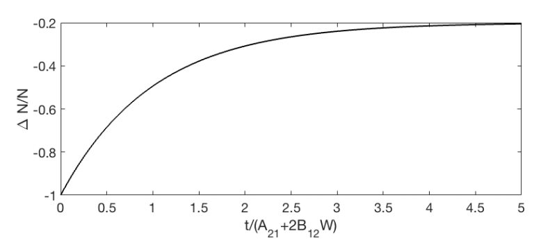
Hence, for \(\Delta N=N_{2}-N_{1}\) : \[\frac{d \Delta N}{d t}=-A_{21} \Delta N-2 \Delta N B_{12} W(\omega)-A_{21} N \nonumber \] where as before: \(N=N_{1}+N_{2}\) is constant. If initially (i.e. at \(t=0\) ) all atoms are in the lowest state: \(\Delta N(t=0)=-N\), then it follows from \(\PageIndex{12}\): \[\Delta N(t)=-N\left[\frac{A_{21}}{A_{21}+2 B_{12} W(\omega)}+\left(1-\frac{A_{21}}{A_{21}+2 B_{12} W(\omega)}\right) e^{-\left(A_{21}+2 B_{12} W(\omega)\right) t}\right] \nonumber \]
An example where \(A_{21} / B_{12} W(\omega)=0.5\) is shown in Figure \(\PageIndex{2}\). We always have \(\Delta N<0\), hence \(N_{2}(t)<N_{1}(r)\) for all times \(t\). Therefore, a system with only two levels cannot have population inversion.
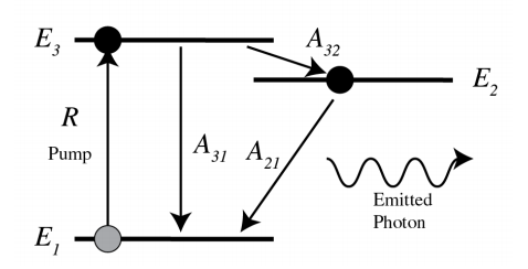
A way to achieve population inversion of levels 1 and 2 and hence amplification of the radiation with frequency \(\omega\) with \(\hbar \omega=E_{2}-E_{1}\) is to use more atomic levels, for example three. In Figure \(\PageIndex{3}\) the ground state is state 1 with two upper levels 2 and 3 such that \(E_{1}<E_{2}<E_{3}\). The transition of interest is still that from level 2 to level 1 . Initially almost all atoms are in the ground state 1 . Then atoms are pumped with rate \(R\) from level 1 directly to level 3 . The transition \(3 \rightarrow 2\) is non-radiative and has high rate \(A_{32}\) so that level 3 is quickly emptied and therefore \(N_{3}\) remains small. State 2 is called a metastable state, because the residence time in the metastable state is for every atom relatively long. Therefore its population tends to increase, leading to population inversion between the metastable state 2 and the lower ground state 1 (which is continuously being depopulated by pumping to the highest level).
Note that \(A_{31}\) has to be small, because otherwise level 1 will quickly be filled, by which population inversion will be stopped. This effect can be utilised to obtain a series of laser pulses as output, but is undesirable for a continuous output power.
Pumping may be done optically as described, but the energy to transfer atoms from level 1 to level 3 can also be supplied by an electrical discharge in a gas or by an electric current. After the pumping has achieved population inversion, initially no light is emitted. So how does the laser actually start? Lasing starts by spontaneous emission. The spontaneously emitted photons stimulate emission of the atoms in level 2 to decay to level 1 , while emitting a photon of energy \(\hbar \omega\). This stimulated emission occurs in phase with the exciting light and hence the light continuously builds up coherently, while it is bouncing back and forth between the mirrors of the resonator. One of the mirrors is slightly transparent and in this way some of the light is leaking out of the laser.