3.6: Spherically-symmetric Systems- Brute Force Approach

Now let us proceed to the mathematically more involved, but practically even more important case of the 3D motion, in a spherically-symmetric potential \[U(\mathbf{r})=U(r) .\] Let us start, again, with solving the eigenproblem for a rigid rotator - now a spherical rotator, i.e. a particle confined to move on the spherical surface of radius \(R\). The rotator has two degrees of freedom because its position on the surface is completely described by two coordinates - say, the polar angle \(\theta\) and the azimuthal angle \(\varphi\). In this case, the kinetic energy we need to consider is limited to its angular part, so that in the Laplace operator in spherical coordinates 66 we may keep only those parts, with fixed \(r=R\). Because of this, the stationary Schrödinger equation becomes \[-\frac{\hbar^{2}}{2 m R^{2}}\left[\frac{1}{\sin \theta} \frac{\partial}{\partial \theta}\left(\sin \theta \frac{\partial}{\partial \theta}\right)+\frac{1}{\sin ^{2} \theta} \frac{\partial^{2}}{\partial \varphi^{2}}\right] \psi=E \psi .\] (Again, we will attach indices to \(\psi\) and \(E\) in a minute.) With the natural variable separation, \[\psi=\Theta(\theta) \mathcal{7}(\varphi),\] Eq. (156), with all terms multiplied by \(\sin ^{2} \theta / \Theta \mathcal{7}\), yields \[-\frac{\hbar^{2}}{2 m R^{2}}\left[\frac{\sin \theta}{\Theta} \frac{d}{d \theta}\left(\sin \theta \frac{d \Theta}{d \theta}\right)+\frac{1}{7} \frac{d^{2} 7}{d^{2} \varphi}\right]=E \sin ^{2} \theta .\] Just as in Eq. (143), the fraction \(\left(d^{2} 7 / d x^{2}\right) / 7\) may be a function of \(\varphi\) only, and hence has to be constant, giving Eq. (144) for it. So, with the same periodicity condition (145), the azimuthal functions are expressed by (146) again; in the normalized form, \[\mathcal{Z}_{m}(\varphi)=\frac{1}{(2 \pi)^{1 / 2}} e^{i m \varphi} .\] With that, the fraction \(\left(d^{2} \not / d \varphi^{2}\right) / 7\) in Eq. (158) equals \(\left(-m^{2}\right)\), and after the multiplication of all terms of that equation by \(\Theta / \sin ^{2} \theta\), it is reduced to the following ordinary linear differential equation for the polar eigenfunctions \(\Theta(\theta)\) : \[-\frac{1}{\sin \theta} \frac{d}{d \theta}\left(\sin \theta \frac{d \Theta}{d \theta}\right)+\frac{m^{2}}{\sin ^{2} \theta} \Theta=\varepsilon \Theta, \quad \text { with } \varepsilon \equiv E / \frac{\hbar^{2}}{2 m R^{2}}\] It is common to recast it into an equation for a new function \(P(\xi) \equiv \Theta(\theta)\), with \(\xi \equiv \cos \theta\) : \[\frac{d}{d \xi}\left[\left(1-\xi^{2}\right) \frac{d P}{d \xi}\right]+\left[l(l+1)-\frac{m^{2}}{1-\xi^{2}}\right] P=0\] where a new notation for the normalized energy is introduced: \(l(l+1) \equiv \varepsilon\). The motivation for such notation is that, according to the mathematical analysis of Eq. (161) with integer \(m, 67\) it has solutions only if the parameter \(l\) is an integer: \(l=0,1,2, \ldots\), and only if that integer is not smaller than \(|m|\), i.e. if \[-l \leq m \leq+l \text {. }\] This fact immediately gives the following spectrum of the spherical rotator’s energy \(E\) - and, as we will see later, the angular part of the energy of any spherically-symmetric system:

\[E_{l}=\frac{\hbar^{2} l(l+1)}{2 m R^{2}}\] so that the only effect of the magnetic quantum number \(m\) here is imposing the restriction (162) on the non-negative integer \(l\) - the so-called orbital quantum number. This means, in particular, that each energy \((163)\) corresponds to \((2 l+1)\) different values of \(m\), i.e. is \((2 l+1)\)-degenerate.

To understand the nature of this degeneracy, we need to explore the corresponding eigenfunctions of Eq. (161). They are naturally numbered by two integers, \(m\) and \(l\), and are called the associated Legendre functions \(P_{l}^{m}\). (Note that here \(m\) is an upper index, not a power!) For the particular, simplest case \(m=0\), these functions are the so-called Legendre polynomials \(P_{1}(\xi) \equiv P_{1}^{0}(\xi)\), which may be defined as the solutions of the following Legendre equation, resulting from Eq. (161) at \(m=0\) : \[\frac{d}{d \xi}\left[\left(1-\xi^{2}\right) \frac{d}{d \xi} P\right]+l(l+1) P=0\] but also may be calculated explicitly from the following Rodrigues formula: 68 \[P_{l}(\xi)=\frac{1}{2^{l}} l ! \frac{d^{l}}{d \xi^{l}}\left(\xi^{2}-1\right)^{l}, \quad l=0,1,2, \ldots .\] Using this formula, it easy to spell out a few lowest Legendre polynomials: \[P_{0}(\xi)=1, \quad P_{1}(\xi)=\xi, \quad P_{2}(\xi)=\frac{1}{2}\left(3 \xi^{2}-1\right), \quad P_{3}(\xi)=\frac{1}{2}\left(5 \xi^{3}-3 \xi\right), \ldots,\] though such explicit expressions become bulkier and bulkier as \(l\) is increased. As these expressions (and Fig. 19) show, as the argument \(\xi\) is increased, all these functions end up at the same point, \(P_{l}(+1)=+1\), while starting at either at the same point or at the opposite point: \(P_{l}(-1)=(-1)^{l}\). On the way between these two end points, the \(l^{\text {th }}\) polynomial crosses the horizontal axis exactly \(l\) times, i.e. Eq. (164) has \(l\) roots. \({ }^{69}\)

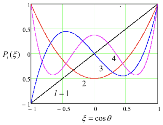Fig. 3.19. A few lowest Legendre polynomials.

It is also easy to use the Rodrigues formula (165) and the integration by parts to show that on the segment \(-1 \leq \xi \leq+1\), the Lagrange polynomials form a full orthogonal set of functions, with the following normalization rule: \[\int_{-1}^{+1} P_{l}(\xi) P_{l^{\prime}}(\xi) d \xi=\frac{2}{2 l+1} \delta_{l l^{\prime}}\] For \(m>0\), the associated Legendre functions (now not necessarily polynomials!), may be expressed via the Legendre polynomials (165) using the following formula: \({ }^{70}\) \[P_{l}^{m}(\xi)=(-1)^{m}\left(1-\xi^{2}\right)^{m / 2} \frac{d^{m}}{d \xi^{m}} P_{l}(\xi),\] while the functions with a negative magnetic quantum number may be found as \[P_{l}^{-m}(\xi)=(-1)^{m} \frac{(l-m) !}{(l+m) !} P_{l}^{m}(\xi), \quad \text { for } m>0 .\] On the segment \(-1 \leq \xi \leq+1\), the associated Legendre functions with a fixed index \(m\) form a full orthogonal set, with the normalization relation, \[\int_{-1}^{+1} P_{l}^{m}(\xi) P_{l^{\prime}}^{m}(\xi) d \xi=\frac{2}{2 l+1} \frac{(l+m) !}{(l-m) !} \delta_{l l^{\prime}},\] which is evidently a generalization of Eq. (167) for arbitrary \(m\).

Since the difference between the angles \(\theta\) and \(\varphi\) is to large extent artificial (due to an arbitrary direction of the polar axis), physicists prefer to use not the functions \(\Theta(\theta) \propto P_{l}^{m}(\cos \theta)\) and \(\mathcal{Z}_{m}(\varphi) \propto e^{i m \varphi}\) separately, but normalized products of the type (157), which are called the spherical harmonics: \[Y_{l}^{m}(\theta, \varphi) \equiv\left[\frac{(2 l+1)}{4 \pi} \frac{(l-m) !}{(l+m) !}\right]^{1 / 2} P_{l}^{m}(\cos \theta) e^{i m \varphi}\] The specific front factor in Eq. (171) is chosen in a way to simplify the following two expressions: the relation of the spherical harmonics with opposite signs of the magnetic quantum number, \[Y_{l}^{-m}(\theta, \varphi)=(-1)^{m}\left[Y_{l}^{m}(\theta, \varphi)\right]^{*},\] and the following normalization relation: \[\oint_{4 \pi} Y_{l}^{m}(\theta, \varphi)\left[Y_{l^{\prime}}^{m^{\prime}}(\theta, \varphi)\right]^{*} d \Omega=\delta_{l l} \delta_{m m^{\prime}},\] with the integration over the whole solid angle. The last formula shows that on a spherical surface, the spherical harmonics form an orthonormal set of functions. This set is also full, so that any function defined on the surface, may be uniquely represented as a linear combination of \(Y_{l}^{m}\).

Despite a somewhat intimidating character of the formulas given above, they yield quite simple expressions for the lowest spherical harmonics, which are most important for applications:

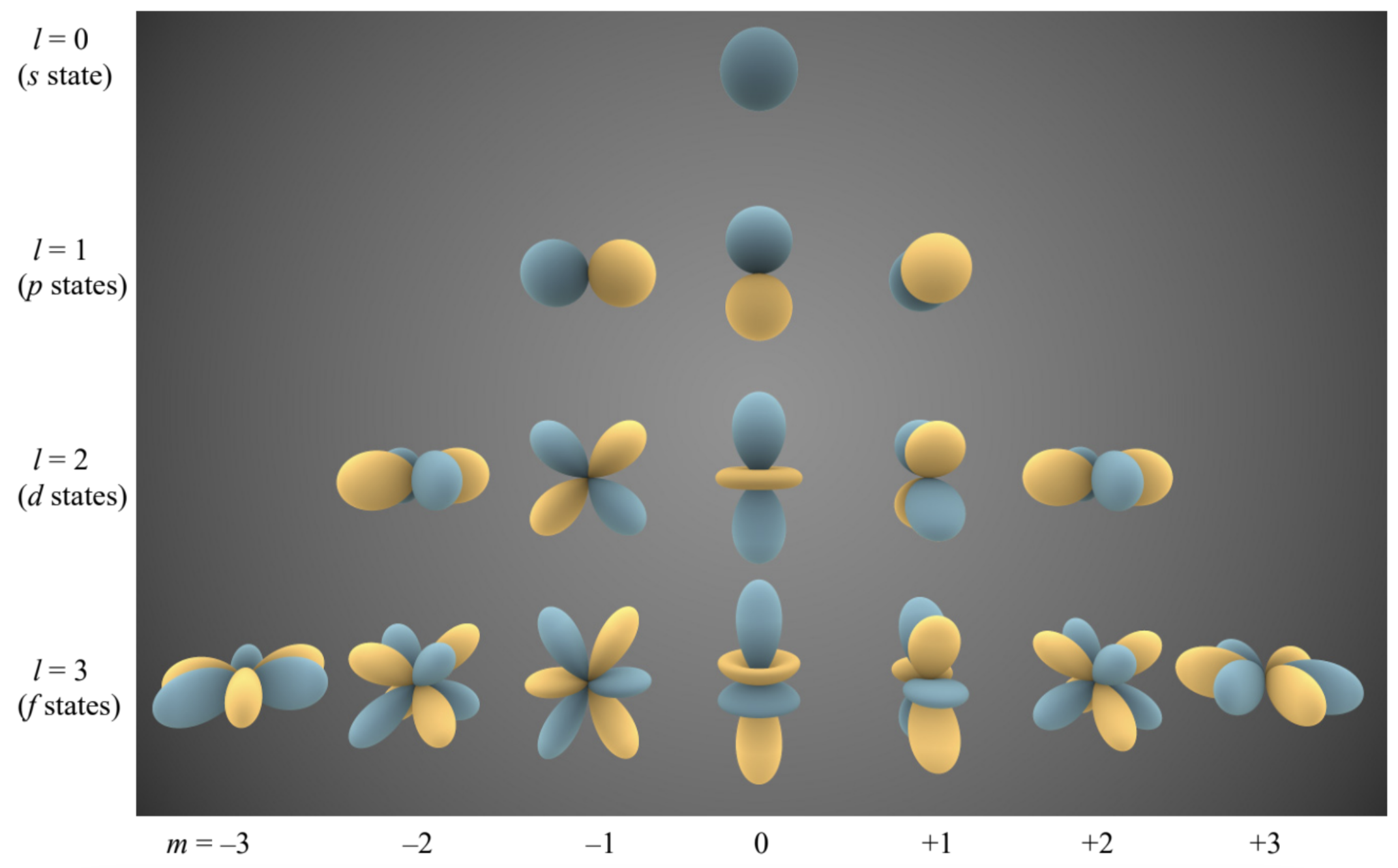
\[\begin{aligned} &l=0: \quad Y_{0}^{0}=(1 / 4 \pi)^{1 / 2}, \\ &l=1:\left\{\begin{array}{l} Y_{1}^{-1}=(3 / 8 \pi)^{1 / 2} \sin \theta e^{-i \varphi} \\ Y_{1}^{0}=(3 / 4 \pi)^{1 / 2} \cos \theta \\ Y_{1}^{1}=-(3 / 8 \pi)^{1 / 2} \sin \theta e^{i \varphi} \end{array}\right. \\ &l=2:\left\{\begin{array}{l} Y_{2}^{-2}=-(15 / 32 \pi)^{1 / 2} \sin ^{2} \theta e^{-2 i \varphi} \\ Y_{2}^{-1}=(15 / 8 \pi)^{1 / 2} \sin \theta \cos \theta e^{-i \varphi}, \\ Y_{2}^{0}=(3 / 16 \pi)^{1 / 2}\left(3 \cos ^{2} \theta-1\right), \\ Y_{2}^{1}=-(15 / 8 \pi)^{1 / 2} \sin \theta \cos \theta e^{i \varphi}, \\ Y_{2}^{2}=(15 / 32 \pi)^{1 / 2} \sin ^{2} \theta e^{2 i \varphi}, \end{array}\right. \end{aligned}\] It is important to understand the general structure and symmetry of these functions. Since the spherical functions with \(m \neq 0\) are complex, the most popular way of their graphical representation is to normalize their real and imaginary parts \(a s^{71}\) \[Y_{l m} \equiv \sqrt{2}(-1)^{m} \times \begin{cases}\operatorname{Im}\left(Y_{l}^{|m|}\right) \propto \sin m \varphi, & \text { for } m<0 \\ \operatorname{Re}\left(Y_{l}^{|m|}\right) & \propto \cos m \varphi, & \text { for } m>0\end{cases}\] (for \(m=0, Y_{l 0} \equiv Y_{l}^{0}\) ), and then plot the magnitude of these real functions in the spherical coordinates as the distance from the origin, while using two colors to show their sign - see Fig. 20 .

Let us start from the simplest case \(l=0\). According to Eq. (162), for this lowest orbital quantum number, there may be only one magnetic quantum number, \(m=0\). According to Eq. (174), the spherical harmonic corresponding to that state is just a constant, so that the wavefunction of this so-called \(s\) state \(^{72}\) is uniformly distributed over the sphere. Since this function has no gradient in any angular direction, it is only natural that the angular kinetic energy (163) of the particle equals zero.

According to the same Eq. (162), for \(l=1\), there are 3 different \(p\) states, with \(m=-1, m=0\), and \(m=+1\) - see Eq. (175). As the second row of Fig. 20 shows, these states are essentially identical in structure and are just differently oriented in space, thus readily explaining the 3 -fold degeneracy of the kinetic energy (163). Such a simple explanation, however, is not valid for the 5 different \(d\) states \((l=2)\), shown in the third row of Fig. 20, as well as the states with higher \(l\) : despite their equal energies, they differ not only by their spatial orientation but their structure as well. All states with \(m=0\) have a nonzero gradient only in the \(\theta\) direction. On the contrary, the states with the ultimate values of \(m(\pm l)\), change only monotonically \(\left(\operatorname{as} \sin ^{\prime} \theta\right)\) in the polar direction, while oscillating in the azimuthal direction. The states with intermediate values of \(m\) provide a gradual transition between these two extremes, oscillating in both directions, stronger and stronger in the azimuthal direction as \(|m|\) is increased. Still, the magnetic quantum number, surprisingly, does not affect the angular energy for any \(l\).

Fig. 3.20. Radial plots of several lowest real spherical harmonics \(Y_{l m}\). (Adapted from https://en.Wikipedia.org/wiki/Spherical harmonics under the CC BY-SA \(3.0\) license.)

Another counter-intuitive feature of the spherical harmonics follows from the comparison of Eq. (163) with the second of the classical relations (152). These expressions coincide if we interpret the constant \[L^{2} \equiv \hbar^{2} l(l+1)\] as the value of the full angular momentum squared, \(L^{2}=|\mathbf{L}|^{2}\) (including its both \(\theta\) and \(\varphi\) components) in the eigenstate with eigenfunction \(Y_{l}^{m}\). On the other hand, the structure (159) of the azimuthal component \(\mathcal{F}(\varphi)\) of the wavefunction is exactly the same as in \(2 \mathrm{D}\) axially-symmetric problems, implying that Eq. (139) still gives correct values \(L_{z}=m \hbar\) for the \(z\)-component of the angular momentum. This fact invites a question: why for any state with \(l>0,\left(L_{z}\right)^{2}=m^{2} \hbar^{2} \leq l^{2} \hbar^{2}\) is always less than \(L^{2}=l(l+1) \hbar^{2} ?\) In other words, what prevents the angular momentum vector to be fully aligned with the axis \(z\) ?

Besides the difficulty of answering this question using the above formulas, this analysis (though mathematically complete), is as intellectually unsatisfactory as the harmonic oscillator analysis in Sec. 2.9. In particular, it does not explain the meaning of the extremely simple relations for the eigenvalues of the energy and the angular momentum, coexisting with rather complicated eigenfunctions.

We will obtain natural answers to all these questions and concerns in Sec. \(5.6\) below, and now proceed to the extension of our wave-mechanical analysis to the 3D motion in an arbitrary sphericallysymmetric potential (155). In this case, we have to use the full form of the Laplace operator in spherical coordinates. \({ }^{73}\) The variable separation procedure is an evident generalization of what we have done before, with the particular solutions of the type \[\psi=R(\rho) \Theta(\theta) 7(\varphi) \text {, }\] whose substitution into the stationary Schrödinger equation yields \[-\frac{\hbar^{2}}{2 m r^{2}}\left[\frac{1}{R} \frac{d}{d r}\left(r^{2} \frac{d R}{d r}\right)+\frac{1}{\Theta} \frac{1}{\sin \theta} \frac{d}{d \theta}\left(\sin \theta \frac{d \Theta}{d \theta}\right)+\frac{1}{\sin ^{2} \theta} \frac{1}{7} \frac{d^{2} 7}{d \varphi^{2}}\right]+U(r)=E .\] It is evident that the angular part of the left-hand side (the two last terms in the square brackets) separates from the radial part, and that for the former part we get Eq. (156) again, with the only change, \(R \rightarrow r\). This change does not affect the fact that the eigenfunctions of that equation are still the spherical harmonics (171), which obey Eq. (164). As a result, Eq. (180) gives the following equation for the radial function \(R(r)\) : \[-\frac{\hbar^{2}}{2 m r^{2}}\left[\frac{1}{R} \frac{d}{d r}\left(r^{2} \frac{d R}{d r}\right)-l(l+1)\right]+U(r)=E .\] Note that no information about the magnetic quantum number \(m\) has crept into this radial equation (besides setting the limitation (162) for the possible values of \(l\) ) so that it includes only the orbital quantum number \(l\).

Let us explore the radial equation for the simplest case when \(U(r)=0\) - for example, to solve the eigenproblem for a 3D particle free to move only inside the sphere of radius \(R\) - say, confined there by the potential \(^{74}\) \[U= \begin{cases}0, & \text { for } 0 \leq r<R \\ +\infty, & \text { for } R<r\end{cases}\] In this case, Eq. (181) is reduced to \[-\frac{\hbar^{2}}{2 m r^{2}}\left[\frac{1}{R} \frac{d}{d r}\left(r^{2} \frac{d R}{d r}\right)-l(l+1)\right]=E \text {. }\] Multiplying both parts of this equality by \(r^{2} R\), and introducing the dimensionless argument \(\xi \equiv k r\), where \(k^{2}\) is defined by the usual relation \(\hbar^{2} k^{2} / 2 m=E\), we obtain the canonical form of this equation, \[\xi^{2} \frac{d^{2} R}{d \xi^{2}}+2 \xi \frac{d R}{d \xi}+\left[\xi^{2}-l(l+1)\right] R=0,\] Satisfied by so-called spherical Bessel functions of the first and second kind, \(j_{l}(\xi)\) and \(y_{(}(\xi) .{ }^{75}\) These functions are directly related to the Bessel functions of semi-integer order, ⁷⁶ \[j_{l}(\xi)=\left(\frac{\pi}{2 \xi}\right)^{1 / 2} J_{l+\frac{1}{2}}(\xi), \quad y_{l}(\xi)=\left(\frac{\pi}{2 \xi}\right)^{1 / 2} Y_{l+\frac{1}{2}}(\xi),\] but are actually much simpler than even the "usual" Bessel functions, such as \(J_{n}(\xi)\) and \(Y_{n}(\xi)\) of an integer order \(n\), because the former ones may be directly expressed via elementary functions: \[\begin{array}{lll} j_{0}(\xi)=\frac{\sin \xi}{\xi}, & j_{1}(\xi)=\frac{\sin \xi}{\xi^{2}}-\frac{\cos \xi}{\xi}, & j_{2}(\xi)=\left(\frac{3}{\xi^{3}}-\frac{1}{\xi}\right) \sin \xi-\frac{3}{\xi^{2}} \cos \xi, \ldots, \\ y_{0}(\xi)=-\frac{\cos \xi}{\xi}, & y_{1}(\xi)=-\frac{\cos \xi}{\xi^{2}}-\frac{\sin \xi}{\xi}, & y_{2}(\xi)=-\left(\frac{3}{\xi^{3}}-\frac{1}{\xi}\right) \cos \xi-\frac{3}{\xi^{2}} \sin \xi, \ldots, \end{array}\] A few lowest-order spherical Bessel functions are plotted in Fig. \(21 .\)

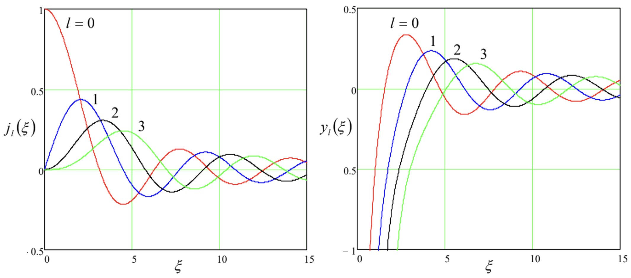Fig. 3.21. Several lowest-order spherical Bessel functions.

As these formulas and plots show, the functions \(y_{l}(\xi)\) are diverging at \(\xi \rightarrow 0\), and thus cannot be used in the solution of our current problem (182), so that we have to take \[R_{l}(r)=\operatorname{const} \times j_{l}(k r) .\] Still, even for these functions, with the sole exception of the simplest function \(j_{0}(\xi)\), the characteristic equation \(j_{l}(k R)=0\), resulting from the boundary condition \(R(R)=0\), can be solved only numerically. However, the roots \(\xi_{l, n}\) of the equation \(j_{(}(\xi)=0\), where the integer \(n(=1,2,3, \ldots)\) is the root’s number, are tabulated in virtually any math handbook, and we may express the eigenvalues we are interested in, \[k_{l, n}=\frac{\xi_{l, n}}{R}, \quad E_{l, n}=\frac{\hbar^{2} k_{l, n}^{2}}{2 m} \equiv \frac{\hbar^{2} \xi_{l, n}^{2}}{2 m R^{2}},\] via these tabulated numbers. The table below lists several smallest roots, and the corresponding eigenenergies (normalized to their natural unit \(E_{0} \equiv \hbar^{2} / 2 m R^{2}\) ), in the order of their growth. It shows a very interesting effect: going up the energy spectrum, first the eigenenergies grow because of increases of the orbital quantum number \(l\), at the same (lowest) radial quantum number \(n=1\), due to the growth of the first roots of functions \(j_{l}(\xi)\), but then suddenly the second root of \(j_{0}(\xi)\) cuts into this orderly sequence, just to be followed by the first root of \(j_{3}(\xi)\). With the further growth of energy, the sequences of \(l\) and \(n\) become even more entangled.

\(l\)	\(n\)	\(\xi_{l, n}\)	\(E_{l, n} / E_{0}=\left(\xi_{l, n}\right)^{2}\)
0	1	\(\pi \approx 3.1415\)	\(\pi^{2} \approx 9.87\)
1	1	\(4.493\)	\(20.19\)
2	1	\(5.763\)	\(33.21\)
0	2	\(2 \pi \approx 6.283\)	\(4 \pi^{2} \approx 39.48\)
3	1	\(6.988\)	\(48.83\)

To complete the discussion of our current problem (182), note again that the energy levels, listed in the table above, are \((2 l+1)\)-degenerate because each of them corresponds to \((2 l+1)\) different eigenfunctions, each with a specific value of the magnetic quantum number \(m\) : \[\psi_{n, l, m}=C_{l, n} j_{l}\left(\frac{\xi_{l, n} r}{R}\right) Y_{l}^{m}(\theta, \varphi), \quad \text { with }-l \leq m \leq+l .\]

---

\({ }^{66}\) See, e.g., MA Eq. (10.9).

\({ }^{67}\) This analysis was first carried out by A.-M. Legendre (1752-1833). Just as a historic note: besides many original mathematical achievements, Dr. Legendre had authored a famous textbook, Éléments de Géométrie, which dominated teaching geometry through the 19th century.

\({ }^{68}\) This wonderful formula may be readily proved by plugging it into Eq. (164), but was not so easy to discover! This was done (independently) by B. O. Rodrigues in 1816, J. Ivory in 1824, and C. Jacobi in \(1827 .\)

\({ }^{69}\) In this behavior, we may readily recognize the "standing wave" pattern typical for all 1D eigenproblems - cf. Figs. \(1.8\) and \(2.35\), as well as the discussion of the Sturm oscillation theorem at the end of Sec. \(2.9\).

\({ }^{70}\) Note that some texts use different choices for the front factor (called the Condon-Shortley phase) in the functions \(P_{l}^{m}\), which do not affect the final results for the spherical harmonics \(Y_{l}^{m}\).

\({ }^{71}\) Such real functions \(Y_{l m}\), which also form a full orthonormal set, and are frequently called the real (or "tesseral") spherical harmonics, are more convenient than the complex harmonics \(Y_{l}^{m}\) for several applications, especially when the variables of interest are real by definition.

\({ }^{72}\) The letter names for the states with various values of \(l\) stem from the history of optical spectroscopy - for example, the letter " \(s\) " used for states with \(l=0\), originally denoted the "sharp" optical line series, etc. The sequence of the letters is as follows: \(s, p, d, f, g\), and then continuing in alphabetical order.

\({ }^{73}\) Again, see MA Eq. (10.9).

\({ }^{74}\) This problem, besides giving a simple example of the quantization in spherically-symmetric systems, is also an important precursor for the discussion of scattering by spherically-symmetric potentials in Sec. 8 .

\({ }^{75}\) Alternatively, \(y_{t}(\xi)\) are called "spherical Weber functions" or "spherical Neumann functions".

\({ }^{76}\) Note that the Bessel functions \(J_{r}(\xi)\) and \(Y_{v}(\xi)\) of any order \(v\) obey the universal recurrent formulas and asymptotic formulas (discussed, e.g., in EM Sec. 2.7), so that many properties of the functions \(j_{i}(\xi)\) and \(y_{(}(\xi)\) may be readily derived from these relations and Eqs. (185).