3.5: Axially-symmetric Systems

I cannot conclude this chapter (and hence our review of wave mechanics) without addressing the exact solutions of the stationary Schrödinger equation \({ }^{53}\) possible in the cases of highly symmetric functions \(U(\mathbf{r})\). Such solutions are very important, in particular, for atomic and nuclear physics, and will be used in the later chapters of this course.

In some rare cases, such symmetries may be exploited by the separation of variables in Cartesian coordinates. The most famous (and rather important) example is the \(d\)-dimensional harmonic oscillator a particle moving inside the potential \[U=\frac{m \omega_{0}^{2}}{2} \sum_{j=1}^{d} r_{j}^{2} .\] Separating the variables exactly as we did in Sec. \(1.7\) for the rectangular hard-wall box (1.77), for each degree of freedom we get the Schrödinger equation (2.261) of a 1D oscillator, whose eigenfunctions are given by Eq. (2.284), and the energy spectrum is described by Eq. (2.162). As a result, the total energy spectrum may be indexed by a vector \(\mathbf{n}=\left\{n_{1}, n_{2}, \ldots, n_{d}\right\}\) of \(d\) independent integer quantum numbers \(n_{j}\) : \[E_{\mathrm{n}}=\hbar \omega_{0}\left(\sum_{j=1}^{d} n_{j}+\frac{d}{2}\right),\] each ranging from 0 to \(\infty\). Note that every energy level of this system, with the only exception of its ground state, \[\psi_{\mathrm{g}}=\prod_{j=1}^{d} \psi_{0}\left(r_{j}\right)=\frac{1}{\pi^{d / 4} x_{0}^{d / 2}} \exp \left\{-\frac{1}{2 x_{0}^{2}} \sum_{j=1}^{d} r_{j}^{2}\right\}\] is degenerate: several different wavefunctions, each with its own different set of quantum numbers \(n_{j}\), but the same value of their sum, have the same energy.

However, the harmonic oscillator problem is an exception: for other central- and sphericallysymmetric problems the solution is made easier by using more appropriate curvilinear coordinates. Let us start with the simplest axially-symmetric problem: the so-called planar rigid rotator (or "rotor"), i.e. a particle of mass \(m,{ }^{54}\) constrained to move along a plane circle of radius \(R\) (Fig. 17) \({ }^{55}\)

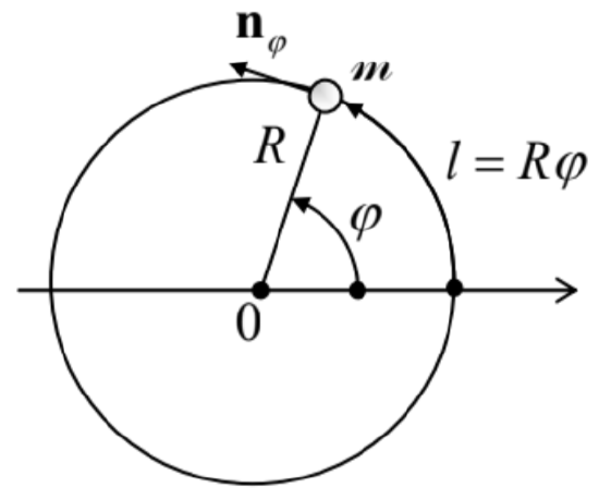Fig. 3.17. A planar rigid rotator.

The classical planar rotator may be described by just one degree of freedom, say the angle displacement \(\varphi\) (or equivalently the arc displacement \(l \equiv R \varphi\) ) from some reference direction, with the energy (and the Hamiltonian function) \(H=p^{2} / 2 m\), where \(\mathbf{p} \equiv m \mathbf{v}=m \mathbf{n}_{\varphi}(d l / d t), \mathbf{n}_{\varphi}\) being the unit vector in the azimuthal direction - see Fig. 17. This function is similar to that of a free 1D particle (with the replacement \(x \rightarrow l \equiv R \varphi\) ), and hence the rotator’s quantum properties may be described by a similar Hamiltonian operator: \[\hat{H}=\frac{\hat{p}^{2}}{2 m}, \quad \text { with } \hat{\mathbf{p}}=-i \hbar \mathbf{n}_{\varphi} \frac{\partial}{\partial l} \equiv-i \frac{\hbar}{R} \mathbf{n}_{\varphi} \frac{\partial}{\partial \varphi},\] whose eigenfunctions have a similar structure: \[\psi=C e^{i k l} \equiv C e^{i k R \varphi} .\] The "only" new feature is that in the rotator, all observables should be \(2 \pi\)-periodic functions of the angle \(\varphi\). Hence, as we have already discussed in the context of the magnetic flux quantization (see Fig. 4 and its discussion), as the particle makes one turn around the central point 0 , its wavefunction’s phase \(k R \varphi\) may only change by \(2 \pi m\), with an arbitrary integer \(m\) (ranging from \(-\infty\) to \(+\infty\) ): \[\psi_{m}(\varphi+2 \pi)=\psi_{m}(\varphi) e^{2 \pi i m} .\] With the eigenfunctions (127), this periodicity condition immediately gives \(2 \pi k R=2 \pi m\). Thus, the wave number \(k\) can take only quantized values \(k_{m}=m / R\), so that the eigenfunctions should be indexed by this magnetic quantum number \(m\) : \[\psi_{m}=C_{m} \exp \left\{i m \frac{l}{R}\right\} \equiv C_{m} \exp \{i m \varphi\}\] and the energy spectrum is discrete: \[E_{m}=\frac{p_{m}^{2}}{2 m}=\frac{\hbar^{2} k_{m}^{2}}{2 m}=\frac{\hbar^{2} m^{2}}{2 m R^{2}} .\] This simple model allows exact analysis of the external magnetic field effects on a confined motion of an electrically charged particle. Indeed, in the simplest case when this field is axially symmetric (or just uniform) and directed normally to the rotator’s plane, it does not violate the axial symmetry of the system. According to Eq. (26), in this case, we have to generalize Eq. (126) as \[\hat{H}=\frac{1}{2 m}\left(-i \hbar \mathbf{n}_{\varphi} \frac{\partial}{\partial l}-q \mathbf{A}\right)^{2} \equiv \frac{1}{2 m}\left(-i \frac{\hbar}{R} \mathbf{n}_{\varphi} \frac{\partial}{\partial \varphi}-q \mathbf{A}\right)^{2} .\] Here, in contrast to the Cartesian gauge choice (44), which was so instrumental for the solution of the Landau level problem, it is beneficial to take the vector potential in the axially-symmetric form \(\mathbf{A}=\) \(A(\rho) \mathbf{n}_{\varphi}\), where \(\rho \equiv\{x, y\}\) is the \(2 \mathrm{D}\) radius-vector, with the magnitude \(\rho=\left(x^{2}+y^{2}\right)^{1 / 2}\). Using the wellknown expression for the curl operator in the cylindrical coordinates, \({ }^{56}\) we can readily check that the requirement \(\nabla \times \mathbf{A}=\mathscr{B} \mathbf{n}_{z}\), with \(\mathscr{R}=\) const, is satisfied by the following function: \[\mathbf{A}=\mathbf{n}_{\varphi} \frac{\mathscr{B} \rho}{2} .\] For the planar rotator, \(\rho=R=\) const, so that the stationary Schrödinger equation becomes \[\frac{1}{2 m}\left(-i \frac{\hbar}{R} \frac{\partial}{\partial \varphi}-q \frac{\mathscr{B R}}{2}\right)^{2} \psi_{m}=E_{n} \psi_{m} .\] A little bit surprisingly, this equation is still satisfied with the eigenfunctions (127). Moreover, since the periodicity condition (128) is also unaffected by the applied magnetic field, we return to the periodic eigenfunctions (129), independent of \(\mathscr{R}\). However, the field does affect the system’s eigenenergies:

\[\begin{aligned} &\text { Planar rotator: } \\ &\text { magnetic } \\ &\text { field's effect } \end{aligned} \quad E_{m}=\frac{1}{\psi_{m}} \frac{1}{2 m}\left(-i \frac{\hbar}{R} \frac{\partial}{\partial \varphi}-q \frac{\mathscr{R} R}{2}\right)^{2} \psi_{m}=\frac{1}{2 m}\left(\frac{\hbar m}{R}-q \frac{\mathscr{B} R}{2}\right)^{2} \equiv \frac{\hbar^{2}}{2 m R^{2}}\left(m-\frac{\Phi}{\Phi_{0}{ }^{\prime}}\right)^{2},\] where \(\Phi \equiv \pi R^{2} \mathscr{B}\) is the magnetic flux through the area limited by the particle’s trajectory, and \(\Phi_{0}{ }^{\prime} \equiv\) \(2 \pi \hbar / q\) is the "normal" magnetic flux quantum we have already met in the AB effect’s context \(-\) see Eq. (34) and its discussion. The field also changes the electric current of the particle in each eigenstate: \[I_{m}=q \frac{\hbar}{2 i m R}\left[\psi_{m}^{*}\left(\frac{\partial}{\partial \varphi}-\frac{i q R \mathscr{R}}{2 \hbar}\right) \psi_{m}-\text { c.c. }\right]=q \frac{\hbar}{m R}\left|C_{m}\right|^{2}\left(m-\frac{\Phi}{\Phi_{0}{ }^{\prime}}\right) .\] Normalizing the wavefunction (129) to have \(W_{m}=1\), we get \(\left|C_{m}\right|^{2}=1 / 2 \pi R\), so that Eq. (135) becomes \[I_{m}=\left(m-\frac{\Phi}{\Phi_{0}{ }^{\prime}}\right) I_{0}, \quad \text { with } I_{0} \equiv \frac{\hbar q}{2 \pi m R^{2}} .\] The functions \(E_{m}(\Phi)\) and \(I_{m}(\Phi)\) are shown in Fig. 18. Note that since \(\Phi_{0}^{\prime} \propto 1 / q\), for any sign of the particle’s charge \(q, d I_{m} / d \Phi<0\). It is easy to verify that this means that the current is diamagnetic for any sign of \(q: 57\) the field-induced current flows in the direction that its own magnetic field tries to compensate for the external magnetic flux applied to the loop. This result may be interpreted as a different manifestation of the \(\mathrm{AB}\) effect. \({ }^{58}\) In contrast to the interference experiment that was discussed in Sec. 1, in the situation shown in Fig. 17 the particle is not absorbed by the detector but travels around the ring continuously. As a result, its wavefunction is "rigid": due to the periodicity condition (128), the quantum number \(m\) is discrete, and the applied magnetic field cannot change the wavefunction gradually. In this sense, the system is similar to a superconducting loop - see Fig. 4 and its discussion. The difference between these systems is two-fold:

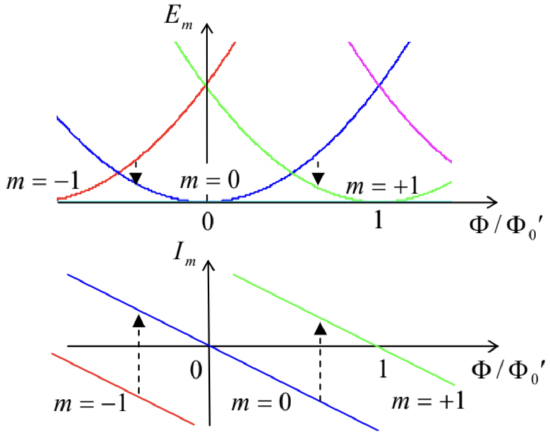Fig. 3.18. The magnetic field effect on a charged planar rotator. Dashed arrows show possible inelastic transitions between metastable and ground states, due to weak interaction with the environment, as the external magnetic field is slowly increased.

(i) For a single charged particle, in macroscopic systems with practicable values of \(q, R\), and \(m\), the scale \(I_{0}\) of the induced current is very small. For example, for \(m=m_{\mathrm{e}}, q=-e\), and \(R=1 \mu \mathrm{m}\), Eq. (136) yields \(I_{0} \approx 3 \mathrm{pA} .{ }^{59}\) With the ring’s inductance \(\mathscr{L}\) of the order of \(\mu_{0} R,{ }^{60}\) the contribution \(\Phi_{I}=\mathscr{L} \sim\) \(\mu_{0} R I_{0} \sim 10^{-24} \mathrm{~Wb}\) of such a small current into the net magnetic flux \(\Phi\) is negligible in comparison with \(\Phi_{0}^{\prime} \sim 10^{-15} \mathrm{~Wb}\), so that the wavefunction quantization does not lead to the constancy of the total magnetic flux.

(ii) As soon as the magnetic field raises the eigenstate energy \(E_{m}\) above that of another eigenstate \(E_{m^{\prime}}\), the former state becomes metastable, and a weak interaction of the system with its environment (which is neglected in our simple model, but will be discussed in Chapter 7) may induce a quantum transition of the system to the lower-energy state, thus reducing the diamagnetic current’s magnitude see the dashed lines in Fig. 18. The flux quantization in superconductors is much more robust to such perturbations. \({ }^{61}\)

Now let us return, once again, to the key Eq. (129), and see what does it give for one more important observable, the particle’s angular momentum \[\mathbf{L} \equiv \mathbf{r} \times \mathbf{p},\] In this particular geometry, the vector \(\mathbf{L}\) has just one component, normal to the rotator plane: \[L_{z}=R p \text {. }\] In classical mechanics, \(L_{z}\) of the rotator should be conserved (due to the absence of external torque), but it may take arbitrary values. In quantum mechanics, the situation changes: with \(p=\hbar k\), our result \(k_{m}=\) \(m / R\) for the \(m^{\text {th }}\) eigenstate may be rewritten as \[\left(L_{z}\right)_{m}=R \hbar k_{m}=\hbar m .\] Thus, the angular momentum is quantized: it may be only a multiple of the Planck constant \(\hbar-\) confirming the N. Bohr’s guess - see Eq. (1.8). As we will see in Chapter 5, this result is very general (though it may be modified by spin effects), and the wavefunctions (129) may be interpreted as eigenfunctions of the angular momentum operator.Let us see whether this quantization persists in more general, but still axial-symmetric systems. To implement the planar rotator in our 3D world, we needed to provide rigid confinement of the particle both in the motion plane and along the \(2 \mathrm{D}\) radius \(\rho\). Let us consider a more general situation when only the former confinement is strict, i.e. to the case when a \(2 \mathrm{D}\) particle moves in an arbitrary centrallysymmetric potential \[U(\boldsymbol{\rho})=U(\rho) .\] Using the well-known expression for the \(2 \mathrm{D}\) Laplace operator in polar coordinates, \({ }^{62}\) we may represent the \(2 \mathrm{D}\) stationary Schrödinger equation in the form \[-\frac{\hbar^{2}}{2 m}\left[\frac{1}{\rho} \frac{\partial}{\partial \rho}\left(\rho \frac{\partial}{\partial \rho}\right)+\frac{1}{\rho^{2}} \frac{\partial^{2}}{\partial \varphi^{2}}\right] \psi+U(\rho) \psi=E \psi \text {. }\] Separating the radial and angular variables as \({ }^{63}\) \[\psi=R(\rho) \mathcal{7}(\varphi),\] we get, after the division of all terms by \(\psi\) and their multiplication by \(\rho^{2}\), the following equation: \[-\frac{\hbar^{2}}{2 m}\left[\frac{\rho}{R} \frac{d}{d \rho}\left(\rho \frac{d R}{d \rho}\right)+\frac{1}{7} \frac{d^{2} f}{d \varphi^{2}}\right]+\rho^{2} U(\rho)=\rho^{2} E .\] The fraction \(\left(d^{2} \mathcal{F} / d \varphi^{2}\right) / 7\) should be a constant (because all other terms of the equation may be functions only of \(\rho\) ), so that for the function \(\mathcal{H}(\varphi)\) we get an ordinary differential equation, \[\frac{d^{2} \mathcal{7}}{d \varphi^{2}}+v^{2} \mathcal{7}=0,\] where \(v^{2}\) is the variable separation constant. The fundamental solutions of Eq. (144) are evidently \(7 \propto\) \(\exp \{\pm i v \varphi\}\). Now requiring, as we did for the planar rotator, the \(2 \pi\) periodicity of any observable, i.e. \[\mathcal{F}(\varphi+2 \pi)=\mathcal{F}(\varphi) e^{2 \pi i m},\] where \(m\) is an integer, we see that the constant \(v\) has to be equal to \(m\), and get, for the angular factor, the same result as for the full wavefunction of the planar rotator \(-\) cf. Eq. (129): \[\mathcal{Z}_{m}=C_{m} e^{i m \varphi}, \quad \text { with } m=0, \pm 1, \pm 2, \ldots\] Plugging the resulting relation \(\left(d^{2} \mathcal{F} / d \varphi^{2}\right) / 7=-m^{2}\) back into Eq. (143), we may rewrite it as \[-\frac{\hbar^{2}}{2 m}\left[\frac{1}{\rho R} \frac{d}{d \rho}\left(\rho \frac{d R}{d \rho}\right)-\frac{m^{2}}{\rho^{2}}\right]+U(\rho)=E .\] The physical interpretation of this equation is that the full energy is a sum, \[E=E_{\rho}+E_{\varphi},\] of the radial-motion part \[E_{\rho}=-\frac{\hbar^{2}}{2 m} \frac{1}{\rho} \frac{d}{d \rho}\left(\rho \frac{d R}{d \rho}\right)+U(\rho) .\] and the angular-motion part \[E_{\varphi}=\frac{\hbar^{2} m^{2}}{2 m \rho^{2}} .\] Now let us recall that a similar separation exists in classical mechanics, \({ }^{64}\) because the total energy of a particle moving in a central field may be represented as \[\begin{gathered} E=\frac{m}{2} v^{2}+U(\rho)=\frac{m}{2}\left(\dot{\rho}^{2}+\rho^{2} \dot{\varphi}^{2}\right)+U(\rho) \equiv E_{\rho}+E_{\varphi}, \\ \text { with } E_{\rho} \equiv \frac{p_{\rho}^{2}}{2 m}+U(\rho), \quad \text { and } E_{\varphi} \equiv \frac{m}{2} \rho^{2} \dot{\varphi}^{2} \equiv \frac{p_{\varphi}^{2}}{2 m} \equiv \frac{L_{z}^{2}}{2 m \rho^{2}} . \end{gathered}\] The comparison of the latter relation with Eqs. (139) and (150) gives us grounds to expect that the quantization rule \(L_{z}=m \hbar\) may be valid not only for this 2D problem but in 3D cases as well. In Sec. 5.6, we will see that this is indeed the case.

Returning to Eq. (147), with our 1D wave mechanics experience we may expect that any fixed \(m\) this ordinary, linear, second-order differential equation should have (for a motion confined to a certain final region of its argument \(\rho\) ) a discrete energy spectrum described by another integer quantum number - say, \(n\). This means that the eigenfunctions (142) and corresponding eigenenergies (148) and \(\mathbb{R} \rho\) ) should be indexed by two quantum numbers, \(m\) and \(n\). So, the variable separation is not so "clean" as it was for the rectangular potential well. Normalizing the angular function 7 to the full circle, \(\Delta \varphi=2 \pi\), we may rewrite Eq. (142) as \[\psi_{m, n}=R_{m, n}(\rho) \mathcal{Z}_{m}(\varphi)=\frac{1}{(2 \pi)^{1 / 2}} R_{m, n}(\rho) e^{i m \varphi} .\] A good (and important) example of an analytically solvable problem of this type is a \(2 \mathrm{D}\) particle whose motion is rigidly confined to a disk of radius \(R\), but otherwise free: \[U(\rho)=\left\{\begin{array}{cl} 0, & \text { for } 0 \leq \rho<R \\ +\infty, & \text { for } R<\rho . \end{array}\right.\] In this case, the solutions \(R_{m, n}(\rho)\) of Eq. (147) are proportional to the first-order Bessel functions \(J_{m}\left(k_{n} \rho\right),{ }^{65}\) with the spectrum of possible values \(k_{n}\) following from the boundary condition \(R_{m, n}(R)=0\). Let me leave a detailed analysis of this problem for the reader’s exercise.

---

\({ }^{53}\) This is my best chance to mention, in passing, that the eigenfunctions \(\psi_{n}(\mathbf{r})\) of any such problem do not feature the instabilities typical for the deterministic chaos effects of classical mechanics - see, e.g., CM Chapter 9. (This is why the term quantum mechanics of classically chaotic systems is preferable to the occasionally used term "quantum chaos".) It is curious that at the initial stages of the time evolution of the wavefunctions of such systems, their certain correlation functions still grow exponentially, reminding the Lyapunov exponents \(\lambda\) of their classical chaotic dynamics. This growth stops at the so-call Ehrefect times \(t_{\mathrm{E}} \sim \lambda^{-1} \ln (S / \hbar)\), where \(S\) is the action scale of the problem - see, e.g., I. Aleiner and A. Larkin, Phys. Rev. \(E 55\), R1243 (1997). In a stationary quantum state, the most essential trace of the classical chaos in a system is an unusual statistics of its eigenvalues, in particular of the energy spectra. We will have a chance for a brief look at such statistics in Chapter 5, but unfortunately, I will not have time/space to discuss this field in much detail. Perhaps the best available book for further reading is the monograph by M. Gutzwiller, Chaos in Classical and Quantum Mechanics, Springer, \(1991 .\)

\({ }^{54}\) From this point on (until the chapter’s end), I will use this exotic font for the particle’s mass, to avoid any chance of its confusion with the impending "magnetic" quantum number \(m\), traditionally used in axiallysymmetric problems.

\({ }^{55}\) This is a reasonable model for the confinement of light atoms, notably hydrogen, in some organic compounds, but I am addressing this system mostly as the basis for the following, more complex problems.

\({ }^{56}\) See, e.g., MA Eq. (10.5).

\({ }^{57}\) This effect, whose qualitative features remain the same for all 2D or 3D localized states (see Chapter 6 below), is frequently referred to as orbital diamagnetism. In magnetic materials consisting of particles with uncompensated spins, this effect competes with an opposite effect, spin paramagnetism - see, e.g., EM Sec. 5.5.

\({ }^{58}\) It is straightforward to check that the final forms of Eqs. (134)-(136) remain valid even if the magnetic field is localized well inside the rotator’s circumference so that its lines do not touch the particle’s trajectory.

\({ }^{59}\) Such weak persistent, macroscopic diamagnetic currents in non-superconducting systems have been experimentally observed by measuring the weak magnetic field induced by the currents, in systems of a large number \(\left(\sim 10^{7}\right)\) of similar conducting rings \(-\) see, e.g., L. Lévy et al., Phys. Rev. Lett. 64, 2074 (1990). Due to the dephasing effects of electron scattering by phonons and other electrons (unaccounted for in our simple theory), the effect’s observation requires submicron rings and millikelvin temperatures.

\({ }^{60}\) See, e.g., EM Sec. 5.3.

\({ }^{61}\) Interrupting a superconducting ring with a weak link (Josephson junction), i.e. forming a SQUID, we may get a switching behavior similar to that shown with dashed arrows in Fig. \(18-\) see, e.g., EM Sec. 6.5.

\({ }^{62}\) See, e.g., MA Eq. (10.3) with \(\partial / \partial z=0\).

\({ }^{63}\) At this stage, I do not want to mark the particular solution (eigenfunction) \(\psi\) and corresponding eigenenergy \(E\) with any single index, because based on our experience in Sec. 1.7, we already may expect that in a 2D problem the role of this index will be played by two integers - two quantum numbers.

\({ }^{64}\) See, e.g., CM Sec. \(3.5\).

\({ }^{65}\) A short summary of properties of these functions, including the most important plots and a useful table of values, may be found in EM Sec. 2.7.